Observation of B0329+54 at 1.42GHz
S56ZSA & S53MV
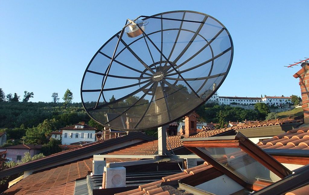
In 2016 we installed a surplus 3.1m-diameter (Echostar 4GHz TVRO) mesh dish on the roof of our house.
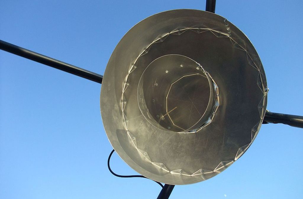
The dish is installed on a surplus AZ/EL rotator EGIS EPR-203 equipped with gears for 360° azimuth range and 90° elevation range. The dish has a f/d ratio of about 0.4 and is equipped with a linearly-polarized VE4MA feed for 1.42GHz. The antenna has a clear view towards south and obstructions (hill with church on top) to the north-east up to an elevation of 15°.
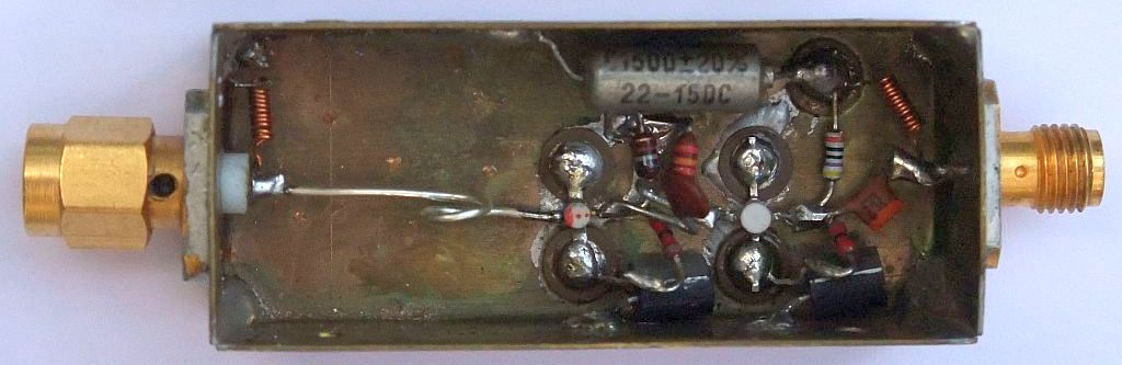
The two-stage HEMT LNA is home-made and is installed directly on the feed. It achieves a noise temperature of around 30K at 1.42GHz as measured with a calibrated HP346A noise head:
The system noise temperature was measured by comparing cold-sky noise to ground (forest) noise. A hot/cold ratio of 7dB was obtained. Estimating the cold sky
temperature Tsky=10K and the ground temperature Tforest=290K, a system noise temperature of Trx=60K is obtained. We estimate that besides the 30K from the LNA, we get an additional 5K from the following receiver stages and some 25K from the feed spillover.
We measured the aperture-illumination efficiency of our reflector as 79% by measuring Sun noise and comparing it to the values reported by at the same time by the observatory in San Vito dei Normanni near Brindisi, Italy
In 2016 we used our antenna to generate a hydrogen map of our galaxy. First we used horizontal polarization and later we switched to vertical polarization. After the LNA we used two home-made three-resonator cavity filters and two additional MMIC amplifiers in front of a DVB-T dongle. The first cavity filter is tuned to equalize the frequency response of the whole system.
This spring 2017 we tried to receive some pulsars thanks to the comprehensive information published on the http://www.neutronstar.joataman.net web page. We decided to start our experiments at 1.42GHz with vertical polarization and use a straightforward wide-band receiver design as explained by Jean-Jacques Maintoux, F1EHN.
We our experiments started with the strongest pulsar B0329+54 visible from the northern hemisphere. The latter is circumpolar from our location and reaches a
maximum elevation of 81.3°. Using vertical polarization we successfully observed B0329+54 shortly after the maximum elevation.
Our present pulsar receiver does not include any frequency conversions. Our pulsar setup only includes amplifiers, filters (20...25MHz bandwidth) and an envelope detector.
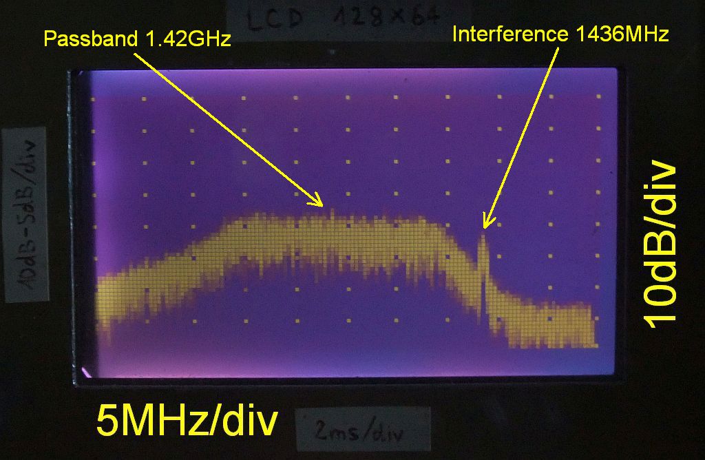
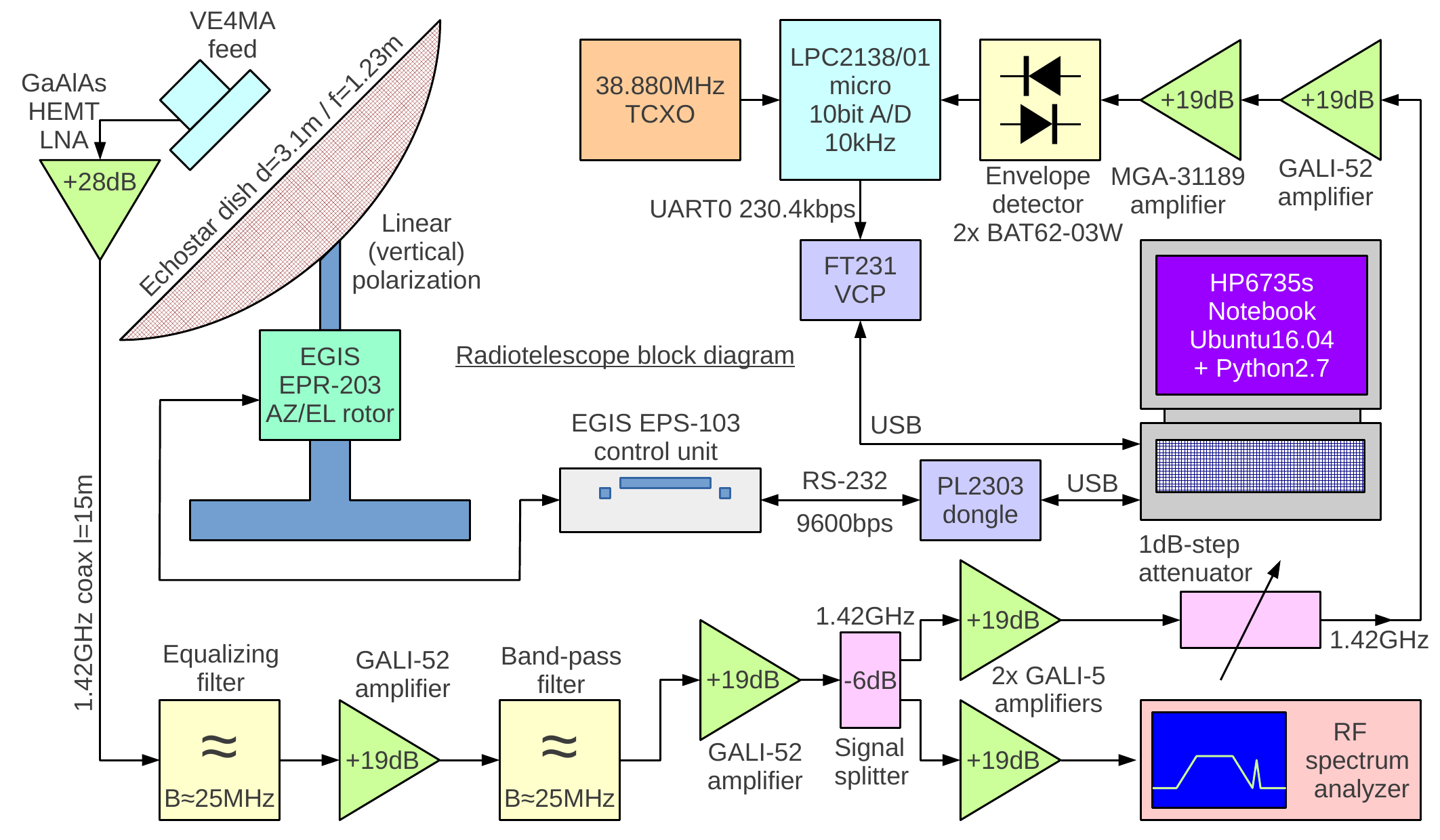 An analog RF spectrum analyzer is connected in parallel to look for interference at all times:
 The envelope signal is sampled at 240kHz with a 10-bit A/D converter. The software running inside the micro-controller LPC2138/01 already decimates this data to a 10kHz sampling rate. To allow precise timing, the 10kHz sampling rate is obtained by dividing the output of a 38.880MHz TCXO (surplus SONET-SDH equipment).
The micro-controller also provides a high-pass filter with a cutoff frequency of about 0.03Hz to remove slow changes of the signal strength like antenna noise- temperature changes with elevation. As large signal changes are removed, small deviations are efficiently encoded in just 8-bit words and transmitter through a virtual USB com port to the notebook computer.
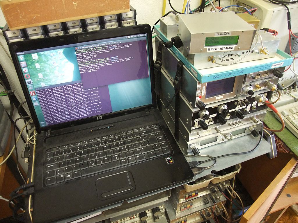
The notebook computer runs two Python scripts: to track the celestial target and to record the incoming data. Usually 200Mbytes of data are collected in one observation resulting in slightly less than 6 hours of observation time:
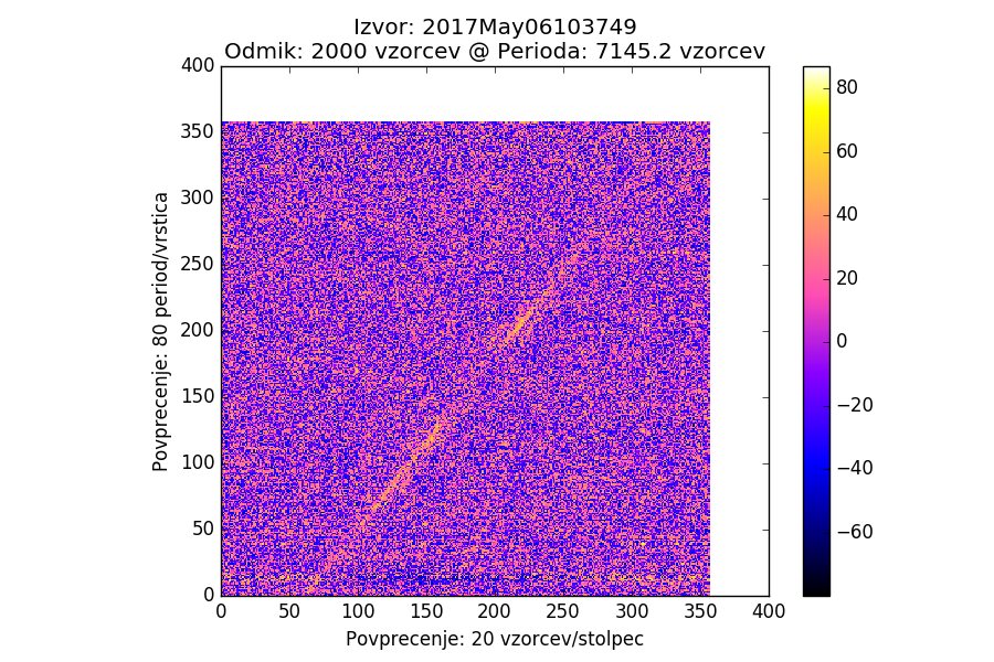
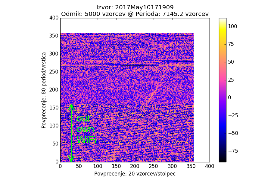
Any further processing is done again using home-made Python scripts on the fastest computer available. First waterfall plots of the 6-hour recordings are made using the nominal pulsar period of 0.71452s as published for the B0329+54 source. 20 consecutive 10kHz data samples are averaged into each column and 80 consecutive pulsar periods are averaged into each row of the waterfall image. We observed severe fading (scintillation) with a period of hours and days on the reception of B0329+54. Any further processing is only done on parts of the recording actually containing useful data on the waterfall. Further, the inclination of the two traces is different showing a significant Doppler change in just 6 days:

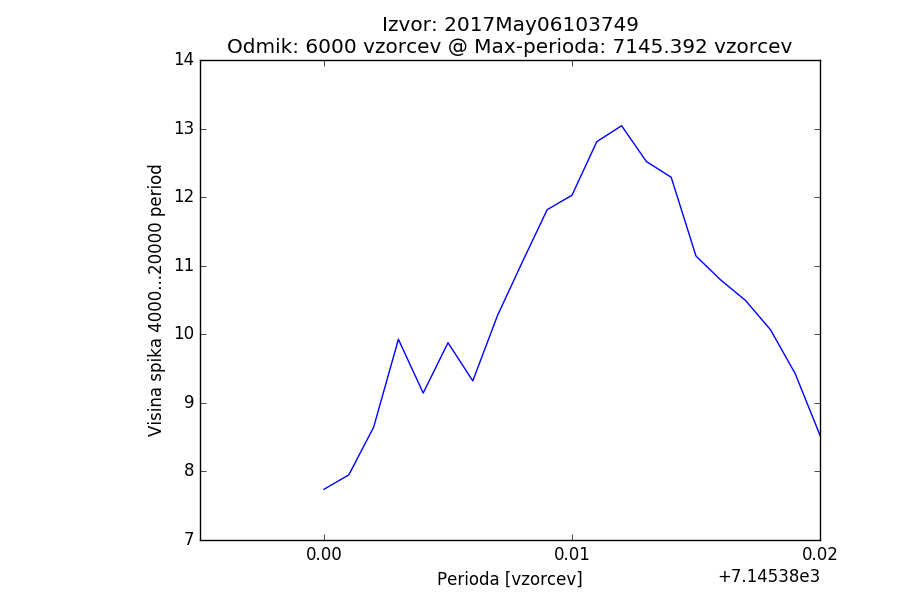
The next step is to find the Doppler correction for the pulsar period. Down to 1ppm this could be done manually. A time-consuming Python script trying different folding periods while looking for the highest correlation peak may be used to get down to about 0.1ppm:
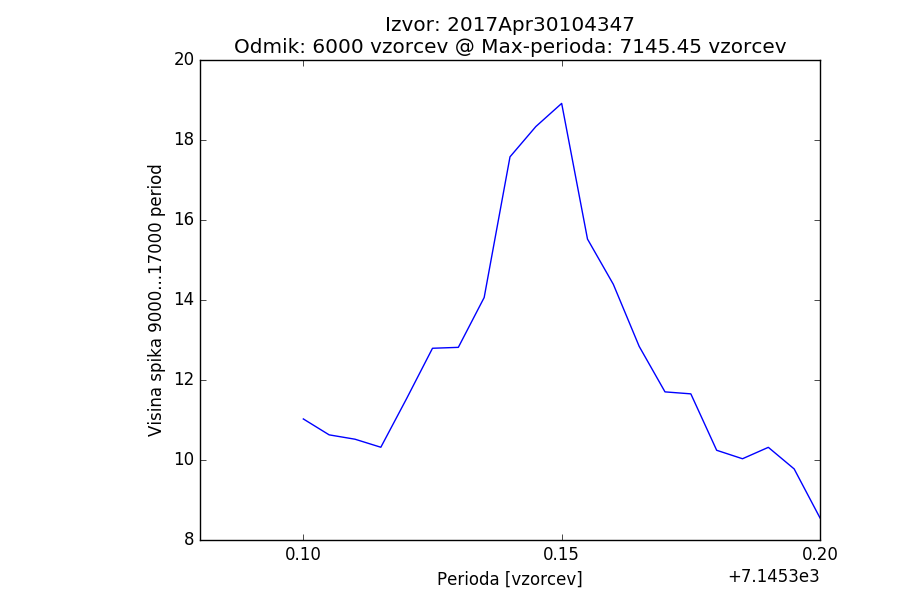
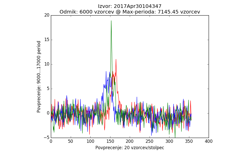
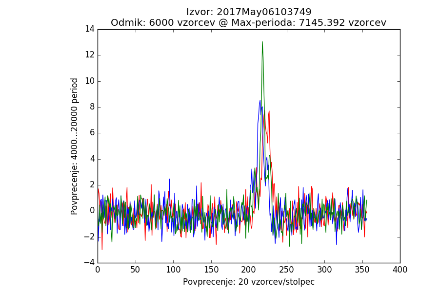
The effect of changing the folding period is clearly visible by plotting the shortest period (red), longest period (blue) and optimum period (green):
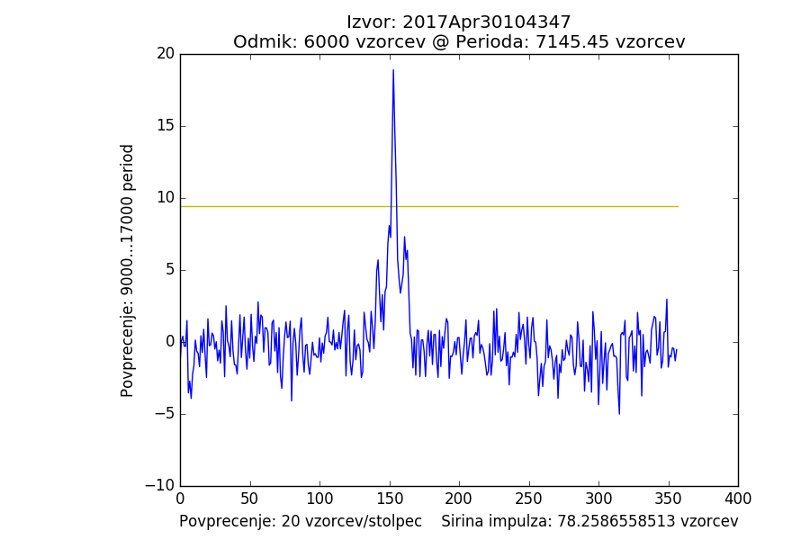
Finally the signal is processed with the optimum folding period and the 50% pulse width is obtained from the measured data:
he same exercise is repeated on the second good recording (6 days later) using a smaller range and a smaller step in the search of the optimum folding period:
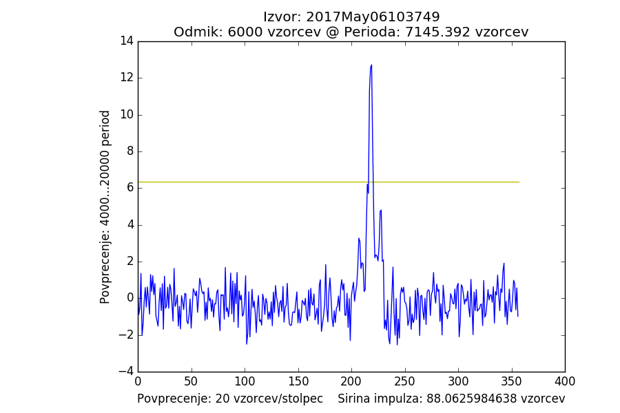
Our measured 50% pulse width for B0329+54 is slightly broader 8...9ms (80...90 samples) than the published data 6.6ms. We suspect that the changing Doppler shift resulting in a curved trace on the waterfall plot is the cause. The expected dispersion broadening is just 1.5ms for our receiver bandwidth.We also tried raised-cosine averaging in place of the simple rectangular averaging in our signal processing obtaining somewhat less noise but even broader pulses. The problem is further complicated by the presence of small leading and trailing pulses well known for B0329+54 and clearly visible on all of our good recordings.
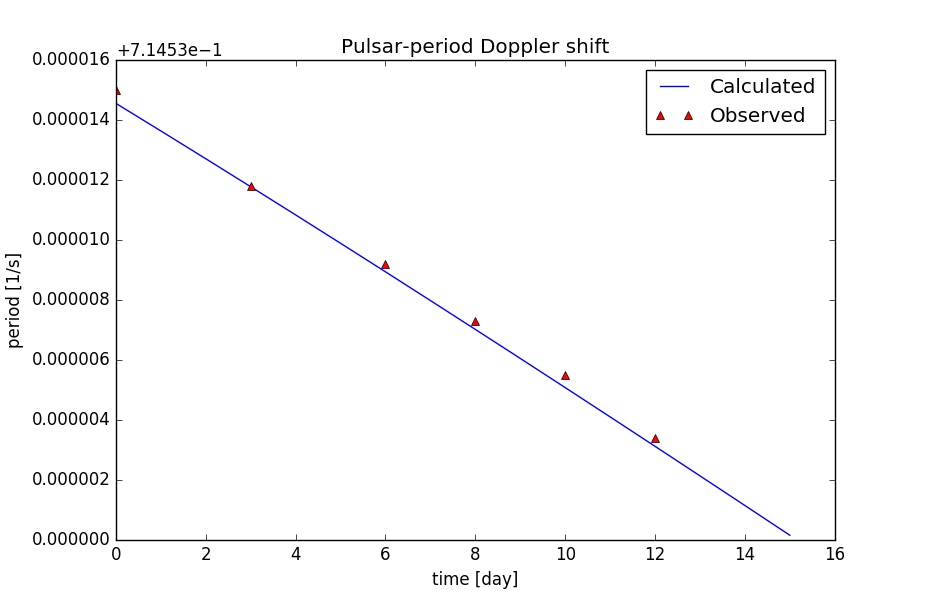
Finally we plotted the measured period (red triangles) against the calculated Doppler shift (blue) for a simple circular orbit of the Earth around the Sun. We intentionally neglected the rotation of the Earth as well as its orbit ellipticity. Unfortunately we do not have data for all days. On some days the signal level was down due to scintillation. On some other days we were simply not at home.
Finally we unintentionally destroyed some data. For example we forgot to turn OFF our home WiFi access point:
Since on favorable days (scintillation) we are able to reliably observe the smaller leading and trailing pulses of B0329+54, we hope to observe some other weaker pulsars with our small antenna in the nearby future as well.