My first idea was to repeat what the guys of the ASTRON Square Kilometer Array team did with their prototype array:
The Phased Array Approach to SKA, Results of a demonstrator project (EXTERNAL LINK),
namely an image of the GPS satellites in the sky.
Why that?
Because the GPS satellites provide several bright point-like quasi-noise sources distributed across the sky.
This has two advantages:
1. Because of their wide angular separation, high resolution is not needed, so small baselines can be used. Basically one can make a "wideangle picture" of the sky.
In this case I decided to simulate a 16x16 array with lambda/2 spacing - this is a total area of 1.5 x 1.5 meters. (GPS C/A operates at cca 20cm wavelength). This would give cca 10 degree pixels in the center of the image (zenith).
2. Because of their brightness, small antennas can be used (typical commercial active GPS antennas are of matchbox size).
The antennas we used looked like this:
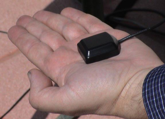
While life was easy for the ASTRON guys who had a fully populated array, we only had a two element interferometer, and had to simulate the array by moving one antena sequentially to every one of the 256 positions.
A very labour intensive way to produce an 0.000256 Megapixel image!!
I estimated the time needed to scan the 16x16 array with cca two seconds of integration at each point plus movement to be cca 15 minutes. The requirement that the satellites don't move much more than one pixel during the "exposure time" thus limited the array size to 16x16 pixels.
I modified the SIDI software for this purpose: sidi11ii.c to record the corellation in a 2^n square matrix. A pushbutton between pins 7 and 8 of the 9-pin COM1 serial port is used to tell the program when the antenna is in position.
This enables a single person to move the antenna and advance the program.
The program beeps once when the button is pressed and again when the measurement at that position is finished, and plays a chord when a row is finished. This way the person moving the antenna doesn't need to watch the screen (which is locked inside a metal box anyway :-)
The program both records the measurements into a file and displays the synthesized image after the whole matrix is scanned.
The image is just a raw 2D FFT of the measured correlation matrix. This gives a certain mapping of the azimuth/elevation coordinates onto the sqaure matrix, comparable to a "circular image fisheye lens" of normal photography:
The elevation circles are at 15 degree intervals (0, 15, 30, 45, 60, 75, and the center point is 90 degrees).
The center point (zenith) is off-center, because the FFT's even size has no "center pixel", so the DC pixel is the first one right and below the center.
The part of the outer circles that "falls out" right and bottom is actually aliased to the left and top rows. (with a lambda/2 spaced array, the waves coming from both ends cause the same 180 deg phase offset between the elements)
The corner elements do not correspond to any physical direction (for example, there is no direction from which a wave could come and cause 180 degree offsets in both rows and columns).
The ASTRON guys decided to cut them off in the above linked article and present circular images. I decided to include the corners, as an indicator of noise and crosstalk in the image (without noise and crosstalk/aliasing they would be black).
To scan the simulated array manually, we drew an 16x16 grid with 10cm spacing on the tarmac in front of Pavle's house, like this:
"R" marks the position of the reference (fixed) antenna, and the scanning sequence is indicated by the numbers and red arrows.
Pavle has made a nice movie of the scanning proces: film_hi.rm (198kB Real Player movie).
The orientation of the final synthesized image depends on the scanning sequence and on many signs and index orders in the software that can all flip the image N/S and/or E/W.
For that reason I did not even try to figure out the image orientation - instead we simply put an artificial reference source up on a ladder:
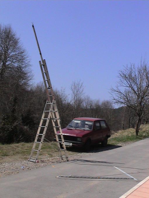
and took a "snapshot", to see where the image of the "artificial star" would fall. On the ground, the square array aperture can be seen, with the reference antenna to the left of the metal rod on which the movable antenna sits. The antenna was magnetic and we pulled it by its cable, the metal rod serving as a guide.
This way we found out that with the above mentioned scanning method and software, south is up and west is right in the final image.
The "artificial star" was a small dipole fed from a 2m transceiver thru a schottky diode to produce some harmonics, of which the 11th was used.
One of the first images of the real sky looked like this:
To reduce the "blockiness" effect, take a few steps back from the monitor.
The dynamic range is 20dB, and there is a kind of "software AGC" that assigns the brightest pixel to pure white.
The hills, trees and the house blocked some of the sky, but at least four satellites are clearly visible, with the fifth on the horizon aliased to both sides of the image.
As far as I know, these are probably the first ever amateur synthesized interferometric images.
Of course, using the knowledge of the GPS spread codes, it would be possible to make an image with a much higher S/N, but that was not my purpose.
What I wanted was to simulate the reception of natural "true noise" sources, which have no deterministic spread code, of course. Therfore I processed the signals without using any knowledge about the GPS spread spectrum codes.
This also shows that an below-noise spread spectrum signal is not really very stealthy - SIDI can not only detect, but also locate it.
Next idea was of course to try recording a movie of the satellites moving across the sky. Since a single scan took 17 minutes, I decided to take a "snap" every 30 minutes.
After three hours the result was this:

For reasons unknown to me, many browsers don't want to display this - to view it in any other program of your choice, download the animated gif file manually here: gpsanim1.gif
As it came out, it is clear that the 30 minute interval was too long - the satellites move too much between the frames and it is very difficult to follow them.
But looking carefully for some time, one can figure out the paths of a few sats, for example two going downwards a little left from the center etc.
Feb 2014: Recalculation of images
After switching from DOS to LINUX, I suddenly had luxurious amounts of memory
at my disposal, so I decided to recalculate the old images.
Basically, I just put the old 16x16 correlation data into the center (low
frequency part) of a bigger 256x256 array, and filled the rest with zeros.
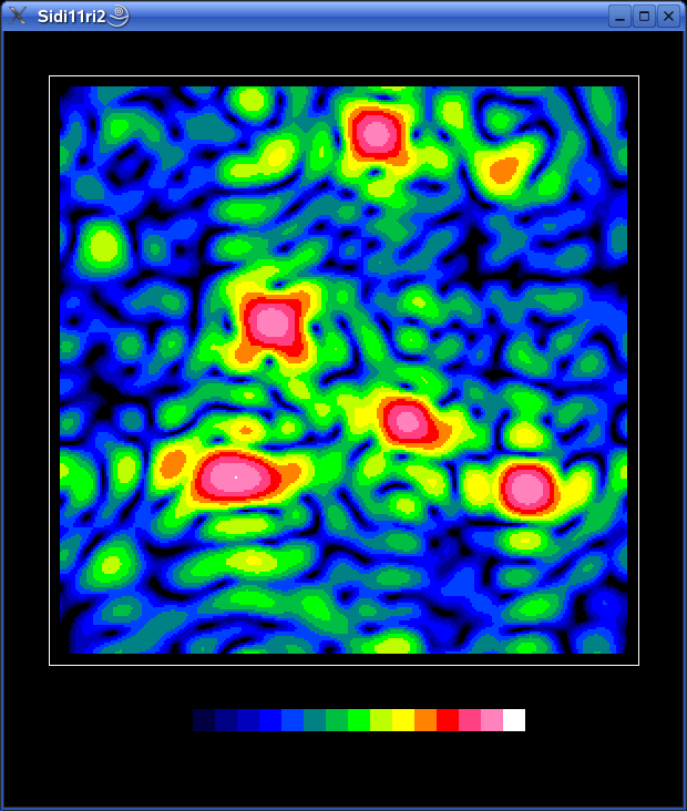
The inverse FFT then produced much smoother results. A frame in false
color now looks like this:
and the animation like this:
I have numbered the sattelites, so it is easier to follow them.
There are also two fixed sources visible, labelled "F". Since they are
down on the horizon (see the fisheye mapping diagram above), they are
most likely terrestrial QRM. Probably the computers we have used...
The C program:
linsidi11ri2.c
Up to main SIDI Page