SIDI version 1.0
Description and results
Hardware description
Software description
Desktop testing
First fringes
More experiments
The Swan caught
First public appearance of SIDI
Planned upgrades and improvements
Harware description, first incarnation:
For the first version (SIDI1.0) I decided to use software timed
sampling. This is not suitable for VLBI, since software loops on
two separate computers will never run coherently, but it allowed
me to test the RF hardware and to get the first fringes. It should
work pretty well for many experiments in connected (non-VLBI)
interferometry, including tests with LO locking etc.
This way I can get a sample rate of cca 600kHz with an 266MHz Pentium
laptop, and still almost 300kHz with an 486/66. The main "brake" here
is the ISA bus to which the LPT port is usually connected.
The basic block diagram of SIDI1 is this:
Since for the first experiments I wnated to try connected (non-VLBI) interferometry, there is
only one LO, power divided into two RF blocks.
The "IF amplifiers" are actually complex baseband amplifiers, but since
they are functionally equivelent to "zero IF" amplifiers, I just call
them that.
For this first incarnation I used mostly modules from the Matjaz Vidmar S53MV's
23cm 1.2Mb/s PSK packet radio transceiver which is described at
S53MV PSK23 description, english (EXTERNAL LINK)
if this link doesn't work an Italian version is at
S53MV PSK23 description, italian (EXTERNAL LINK)
These links contain all the schematics, PCB layouts, component
placements etc.
The downconverter are figs 7 and 8 in the top link (english), the IF amplifier is fig 15 in the same link, and the LO are figs 3,4 and 5
in that link.
The only modification is to the IF amplifiers, where I changed the values
of the input lowpass filter to 1n5, 1.5mH and 2n2, giving a cutoff at
150kHz. These IF amplifiers with their distributed AGC
are much too complex for this application, but I used them because I
had them lying around from some packet radio projects (Matjaz developed
a new IF amp for packet in the meantime, so these were leftovers from
upgrading packet radios).
The outputs of the IF strips go to the "one bit A/D converters",
actually just simple comparators with adjustable thresholds:
Their outputs directly feed the status input bits of the parallel
port on the PC. Pinout is described in the software sources.
Using the S53MV modules allowed me to get "on the air" quickly, since
I had some of them lying around from packet radio projects.
Matjaz designed similar quadrature
I/Q mixers for all amateur bands between 1 and 10GHz, so it would be
possible to make interferometers for 1.3, 2.3, 3.4, 5.7 and 10.4 GHz using
these. However they have limited frequency coverage, for example the 23cm
version doesn't cover the astronomically interesting 21cm band.
Because I would like to avoid that limitation, I am already thinking
about an alternate solution. The modular design will permit changing
only the converter to achieve this. One possibilty would be the tuners
for digital satellite TV, if their LO's could be locked precisely
enough. And I definitely want to try this, since otherwise they are
ideal. Basically they are 0.9 to 2.1GHz quadrature direct conversion
receivers with built in synthesized LO's - just what the doctor
prescribed. I will try to remove the internal reference quartz and
inject an external reference to see if the built in synth has low
enough phase noise.
The whole thing (less the antennas, preamps and laptop PC) looks like this:
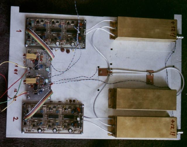
The middle brass box is the LO, which via a wilkinson divider made
from cables, feeds the two converter boxes on the sides. This LO was
designed to feed only one of the converters, but by using diode pairs instead
of quads, I reduced the LO power requirement by 6dB, so one LO module
can easily feed two converters. (BAT 14-099R are almost imposiible to
get anyway)
The I and Q signals from these go to the IF amplifiers (the PCBs
with the three DIPs in the middle), and from there to the comparator
board (the mess on the holematrix board in the middle).
A closeup of the LO and one converter box open look like this:
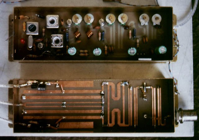
In the LO box on top, the quartz is on the left, and the multiplier
stages go to the right.
The converter box has the RF input on the right (BNC), which goes
to a printed interdigital bandpass, an MMIC amp, another bandpass,
and then to the quadrature hybrid feeding the mixer diodes.
On the left, in the middle is the in-phase LO divider and on the sides
some stubs to provide the required impedances to the mixer diodes.
The few components on the left top and bottom are the first stage of
IF amplification.
Software description, first incarnation:
Since in this first version I rely on software loop timing, I choose
DOS, where by disabling the 17ms system clock interrupt one can have
uninterrupted loops. Although for simple "first fringes" type experiments
with short baselines uniform sampling is not stricltly neccessary (even
with nonuniform sampling there would still be correlation between the
channels, provided they are sampled simultaneously), I decided to go for
it because it is required for delay equalization, phase rotation etc.
The programs are written in C, intended for the
Borland DOS compiler. They expect the BGI graphics drivers in C:\BC\BGI, otherwise you must change the source.
In the near future I plan to add an FIFO buffer
between the comparator outputs and the LPT port, so it will be
possible to use LINUX on the computer.
These first versions of the programs are still very "experimental",
full of code intended for debugging both the hardware and software,
"orphaned" functions etc.
No attempt was made to give them any nice structure and order, but
that shouldn't be a big problem since the main function mostly
just runs linear from start to end.
The main piece of software is
sidi1.c. When started, it will first coarsely
measure the sample rate (computer speed) and check the quadrature
of the I and Q channels and print out these values.
Press any key
to go to the next stage, where it will print some input samples and
then start outputing the DC offsets. This allows the user to set the
DC offsets as close to zero as possible with the potentiometers on the
comparator board.
After setting the DC offsets (or imediately, if they were set before)
press any key again for the next stage, where the correlation values
are output both in rectangular and polar versions. This is intended
mainly for laboratory tests with solid state noise sources etc, to
quantitatively determine the sensitivity and similar.
Pressing any key from here will switch to the real time correlation
display.
It is a polar display of the complex correlation coefficient:
The scaling is determined by the variable "mer" as assigned in the line
with the comment "scaling factor" (line 296). The rim of the diagram
represents an absolute value of 1/mer.
Again, this mode is mainly useful for desktop testing.
Pressing any key again, the main part of the program will start, where
fringes are drawn and correlation data is stored in a file.
The program will ask for a filename to store the results. No checks
are performed on the input, if you type funny stuff the program will
probably crash. If a file with the given name exists, it will be
overwritten without any warning.
The scaling of the on-screen graph is determined by the variables
"avg", "mer" and "xkor" in the line 323 with the comment "fringe drawing".
"avg" determines how many blocks of samples will be averaged together
to form one point on the plot and one data point in the output file.
The higher the value, the slower the graph will be drawn, but with less
noise.
"mer" determines the top and bottom graph values, similar as in the
real time correllation display.
"xkor" determines the x stepsize on the graph, that is, each data point
will be drawn "xkor" pixels to the right of the previous one. Total
graph width is 512. This helps to draw a full graph faster with high
values of "avg".
Pressing any key during this mode will close the output file and exit
the program.
The program works by sample "blocks". First a sampling function
samples the inputs and packs the bits into an array of 16bit integers.
Because of DOS, the size of this array is limited to 64KB, which can
hold 128K (131072) samples. Each sample is 4 bits: one I and one Q
bit from two channels.
After the array is filled, a function computes the correlation
coefficient for these 128K samples, correcting for the DC offsets in
the channels. A very fast table lookup method of calculation is used,
so that even on an 486 machine correlation takes less time than the
sampling!
After the correlation function, its output is either output directly
or further averaged with results from previous sample blocks. The
program then continues by sampling the next 128K sample block.
The correlation works the following way:
Each channel is represented by two bits, I and Q. It can have four
different states, 00,01,10 and 11, which corespond to signal phases
0, 90, 180 and 270 degrees.
Wtih two channels we have four bits, which give 16 possible combinations.
We are interested only in the relation between the two channels, not
their absolute phases. Since each channel can have the four above
mentioned phases, and considering the periodicity of the phase,
there are four possible mutual relationships:
both channels same phase, channel 1 leads 90 degrees, channel 1 lags
90 degrees, and antiphase channels (180 deg).
How does this relate to
the above mentioned 16 possibilities? Because for example, both
channels can have the same phase four ways: (0,0) (90,90) (180,180) and
(270,270). The same is true for the other three mutual phases too, so we
get 16 combinations.
We assign the correlation value (real=1, imag=0) to the "same phase" case,
(real=0, imag=1) to "ch 1 leads", (real=0, imag=-1) to "ch 1 lags" and
(real=-1,imag=0) to "antiphase channels".
Four samples are packed together into 16 bit integers and the fastest
way to find the sum of the correlation values for these four samples is
to make two tables (real and imag) with 65536 entries each, containig
all the possible correlation sums. This way four samples at a time are
processed by two simple array references. It only remains to sum up
both values for the 32768 integers in the sample block.
I haven't yet applied the Van Vleck correction, since in this phase of
the project I just want to see some fringes and get a general feeling
about how this works :-)
With long baselines, it is often necesarry to do "fringe stopping" to
enable longer integration times. This is done by rotating the phase of
one channel. In our 1-bit I/Q scheme, we can rotate the phase by 4
different amounts: 0, 90, 180 and 270 degrees. Although it would be
simple to manipulate the bits to effect this, the table lookup method
of correlation offers a better solution: generate four different sets
of tables corresponding to four possible rotations. This way phase
rotation can be done simply by swithcing the tables at appropriate times,
enabling us to do fringe stopping at almost zero overhead!
In this version of software I haven't yet implemented this because of
DOS memory limitations and because it is intended for connected
interferometry, where the baselines are not likely to be very long.
There are always some residual DC offsets that would cause false
correlation, so this function also calculates the DC offsets and applies
adequate correction.
For (hardware) debugging purposes I have written two auxiliary programs.
sidi1tdd.c is a time domain display utility.
It displays oscillograms and autocorrelation plots of the four inputs.
The oscillograms are mainly for checking if the inputs are alive at
all, while the autocorrelation plots give an idea about the amount of
oversampling and a check/comparison of the lowpass filters.
The oscillograms should look like random binary signals, and the
autocorrelation plots should be similar to each other, with a main
lobe and some sidelobes, depending on the input filter on the IF amplifier.
For example, on this screenshot of sidi1tdd

it can be seen that the fourth channel (channel 2 Q) is totally dead.
The positions of the maximums of the first sidelobes
show that the first channel has the highest cutoff frequency and the
third the lowest.
sidi1fft.c is a spectrum display utility.
It shows the spectrums of both interferometer channels around the
central frequency. Its main purpose is to check for oscillations in the
hardware and for any narrowband interference. For example I had problems
with magnetic pickup of the switcher supply from the laptop into the coils
of the lowpass filter on the input of the IF amplifier. CRT monitor
horizontal deflection frequencies are also in this range.
It is not much of a spectrum analyzer, because the 1-bit sampling
makes the dynamic range pretty small, and the image rejection is also
no better than cca 15..20 dB, depending on the channel quadrature and
balance, which deteriorates especially around the LP band edge, because
the filters aren't matched very well.
However this does not destroy its weak signal detection capabilities,
and I think this could be a good way towards high bandwidth amateur SETI.
This program is so big that I couldn't fit the DOS screengrabber into
the 640k, so I had to take the screenshot with a digicam:
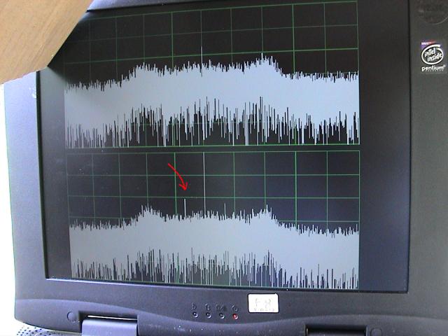
The read arrow shows an interfering signal in the channel 2 (lower trace).
The lines in the middle are caused by the residual DC offset. The 'bumps'
in the noise are an overshot in the frequency
characteristic of the (underdamped) lowpass filters.
I'm not sure why there is not more
difference in the noise levels between the passband (middle) and stopband,
could be that this is just noise aliasing caused by the hard limiting?
Desktop testing:
Since I live in an downtown appartment block, I dont have a suitable
backyard, and the QRM situation is hopeless, so I decided to test the
hardware and software with a lab setup, before going out.
The setup was like this:

Even when I just connected the power splitter, the correlation
coefficient already went up! Unless things were oscillating, this
indicated we have some serious sensitivity here, even without preamps,
since it was just the resistors in the splitter providing correlated
noise.
On the other hand, with the aplified noise source, I expected correlation
close to 1 (I had close to 60dB of ENR, or 300000000K) but it only
came up to cca 0.4 or so. After Van Vleck, this is cca 0.63, so about
2dB short. I still haven't figured out where I loose this, probably
it's in the channel imbalances, like the LP filters not properly
matched - I used 20% ceramic capacitors and was sleepy when winding
the coils....
Next I tried phase measurement, the very essence of interferometry,
by inserting cca 90 degrees of delay into one or the other channel.
I simply used a MM and FF BNC adapter in series:

which gave me cca 100 degrees of phase shift. The little cross on the
real time correlation display moved accordingly, and I was very happy.
First fringes:
Even before I had ironed out all hardware bugs
and quirks, I couldn't resist the temptation, after playing for
months with a solid state noise source and pieces of cable,
to show some real sky to this baby.
Because I use a fixed, multiplied crystal LO, I can't evade
potential interference, I asked Pavle S57RA to do the tests
at his place, because he lives in a pretty secluded valley.
Even there, we still had to put up with some nasty "jammer" signal,
which almost prevented us from getting any results...
The signal definitely came in through the antennas, but Pavle
later mentioned it could be also LO intrusion (as you can se on the photos
above, there was very little shielding) - we will need to check this out.
Another possibility are military aviation spread spectrum links, since
the Aviano air base was relatively close (~100km).
Or was it the revenge from the Slovenian packed radio system, from
where most of the hardware was alienated? :-)
How should i say... the battle was bloody but the victory sweet :-)
The setup looked like this:
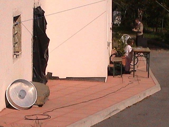
Here both antennas can be seen, the receivers and laptop are
on the table where one of Pavle's daughters is inspecting them.
Antennas were two short backfire 16dBi antennas, also from
the S53MV's packet radio system. 16dBi is approximately
equivalent to a cca 1 meter long yagi on this frequency. Such a yagi
is much smaller and lighter than a SBFA, but has higher sidelobes.
Preamps were the S53MV's small L-band type, with cca 50K of
noise on this frequency (1276.88 MHz, 288 times color carrier) so
I reckon total system temp was probably below 100K, except when
looking through trees :-)
The goal was to get some fringes from the Sun.
There were big problems with the jammer signal, but
heavily increasing the averaging finally allowed me to see
some fringes:
This is cca 1 hour worth
of observation, the amplitude of the fringes is diminishing because
the Sun is getting out of the antenna's cca 30 degree main beam.
The noise on the waveform is 99% external, without the jammer the
curves would be almost perfectly smooth sinusoids. White is real
and red is imaginary component of the correlation coefficient.
Baseline here was cca 5..6m approx east-west. The averaging was set to
100, which means each data point was calculated from 13 million input
samples.
The output file corresponding to this graph is
sun13
The clock on my laptop was several hours off, so you can ignore the
timestamps on the screenshots...
Later the jammer was a little weaker for some time (see the first two
divisions below),
but here I had some hardware
problems, as you can see from the DC offsets on the curves.
The wiggles in the curves in divisions 3 and 4 are the results of my
"massaging" of the hardware to get the gremlins out, but just as I was
getting some success, the jammer intensified again (division 5).
All I could do then is to reduce the baseline to stretch out the fringes.
Anyway, these first two divisions give a taste of how nicely this can
work.... For some time the jammer was low enough so that by holding
one antenna like this
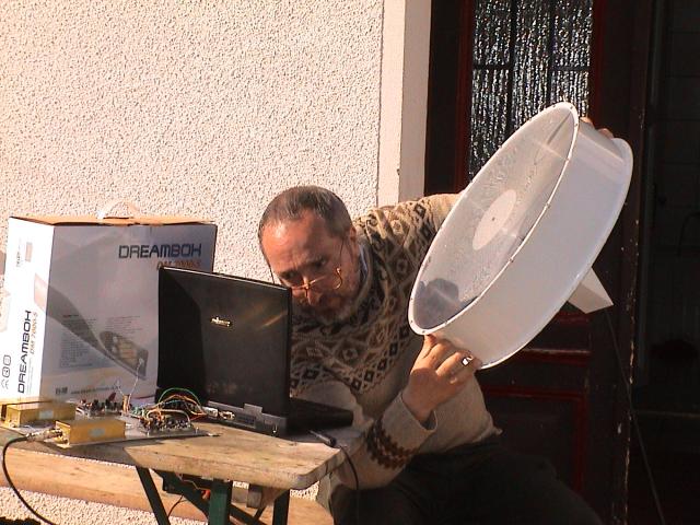
and moving it to and fro (closer and farther from the Sun) for a
wavelength or so, I could watch the phase change on the real time correlation display
(MPEG movie, 1.3MB)
The only function of the dreambox is to cast some shadow onto the
computer's display.
More experiments
After the urge to see the first fringes was satisfied, it was time for
more debugging and to try and get some quantiatative results.
Last weekend (6 June 2004) I visited Pavle again and we did some
debugging work on SIDI. First we improved shielding by putting
everything into a metal box. Then we found and eliminated (I hope!) a
bug that caused one of the channels to intermittently stop working.
After that we set up the same antennas as the last time,
aimed them at the Sun and were elated to see some slick curves
like these:

And this with averaging set to 10 (ten times lower than for the
first fringes above, note the horizontal scale!)
Later we found out that while
the shielding did help, the main reason this worked so swell was that
it was a Sunday and the jammer had a day off. Well, not quite, every
couple of hours or so it still came on for several minutes as can be
seen
here (GIF image 17kB)
The baseline was cca 16m, azimuth cca 100deg, and set on a slightly
sloping terrain, so the west antenna (channel 2) was maybe 1m higher.
16m was the distance between the antennas, the effective baseline was
shorter because of the Sun's angle, as can be estimated from the fringe
period.
A simple method to quickly
estimate fringe frequencies is this: first calculate the "one second
baseline" which is wavelength/7.27E-5, in our case cca 3200m. The
funny number in the denominator is just the angular velocity of Earth
rotation. Then for example, if the baseline is 20m, this is 1/160
of the "one second baseline", and the fringe period will be 160s.
In the above picture, the period is cca 340 sec, so the effective
projected baseline was 3200/340, some 9.5 meters.
Again, the timestamps are bogus. I switch off the system clock interrupt,
so the system clock stands still most of the time.
The measured fringe amplitude is cca +- 5%. Applying the Van Vleck
correction, this gives a correlation coefficient of 7.8%.
With 100K system noise this would
be 7.8K of noise contribution from the Sun. The SBFA's beamwidth is cca
30 deg, so the Sun (0.5 degree) covers cca 1/3600 of the main beam
solid angle.
This gives 28000K, and adding the other polarization 56000K.
The 10cm flux on this day was cca 88 SFU (8.8E5Jy).
The corresponding temperature for a 0.5 degree disk is cca 40000K.
On 23 cm, it was probably more than 100000K, so there are cca 3dB missing.
Apart from the missing two dB that I noticed already during the desktop
testing, the rest is
probably due to antenna pointing and polarization errors and antenna gain
deviation. It could also be that the system noise temperature was
somewhat higher, because the antennas were surrounded by many 300K
objects like the house and trees. Especially the trees were sometimes
quite near the antenna beam.
I find a dB or two of discrepancy still pretty good for a system
that was just put up like that, no calibration etc.
The Sun's angular diameter is cca 0.5 degree or 1/100 radian, so it
should start to be resolved at baselines of cca 100 wavelengths, 23m
in our case. Theoretically an uniformly illuminated circular disk has
a visibility function defined by Bessel functions similar to a sinx/x
shape, with a main lobe, diminishing sidelobes and nulls between them.
For a 0.5 degree disk, the first null should be at cca 94 wavelengths.
As we expanded the baseline, the fringes started to shrink at cca 30m,
and at cca 35m they were like this:

The period of the fringes here is cca 150 sec, so the effective
projected baseline was cca 21 meters. (The horizontal scale value
of 120.9 sec/div is very coarse, could be +-20%, because that's the
precision with which the "checkspeed" function measures the speed of
the computer - and all timing here depends on software loops)
With still larger baselines, the fringes started to grow again,
for example at cca 50m:

which was the end of our cable :-)
Of course there are some errors in the recorded fringe visibilities
(amplitudes) because of antenna pointing and polarization errors,
but the dip in the fringe visibility was definitely there, and this
could be considered as the first 'real' quantitative result of SIDI:
measuring the angular size of the Sun.
The antennas were "mounted" like this:

so the phase of the fringes was not really calibrated and I cannot
say if the phase flipped between the lobes...
Of course, the Sun is not an uniformly illuminated disk (two days later
when watching the Venus transit, I saw two sunspots smack in the middle)
so the nulls aren't very deep etc etc...
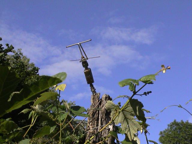
The silky smoothness of the fringes made me bold enough to try something
I calculated before should be possible but was shy to try...
So I asked Pavle to make two small dipole antennas, here he's holding them:

probably among the smallest antennas ever used for radio astronomy?
After increasing the averaging to 100 and setting up a short baseline,
the fringes were clearly visible, at least until the jammer switched on again:
The horizontal scale was in fact cca 600sec/div (the program did not
take into account xkor=2 - a bug in the printout).
The S/N of the fringes was quite good (note the increased vertical
scale) despite the fact that, because of the broad antenna patterns,
the system noise was much higher than the usual 100K.
Some of the distortion in the fringe's shape is probably due to ground
and other reflections which were able to enter the antenna's broad
directional pattern, even with some green absorber around the antennas:
The small brass box is the LNA and the slanted piece of UT141 soldered
to the flange of the N connector acts as a balun.
The DC offsets of the fringe curves are probably the result of LO
amplitude noise being detected in the mixer diodes, causing some fixed
amount of correlation.
If so, in an VLBI setup it will automatically disappear, because
the noise of two separate oscillators won't be correlated.
Otherwise, this should be easy to get rid off by simple "DC removal".
Another possibility is that these offsets are caused by a very weak
terrestrial signal that comes into both antennas with fixed phase.
The amplitude of the fringes is 0.2%, 25 times or 14dB less than with
the SBFA. This is 3dB more than the 11dB gain difference alone
(SBFA 16dBi, dipole with reflector 5dBi), probably because of the
higher system noise temperature with the broad antennas.
Anyway, seeing the fringes with antennas like these really made me feel
good - imagining what could be done with some 'real' antennas!
The Swan caught
After the Sun, the desire was of course to observe something "less local".
A study of radio catalogues has shown that the radio galaxy in Cygnus would
be the best candidate - it is very radio bright and located conveniently
high in the sky in the northern summer nights. (For QRM reasons night time is
preferred. It is also easier to aim the antennas if you see the stars, and
last but not least, since most of the observation consists of waiting, beer
drinking with friends is a suitable auxiliary activity, and that is also
somehow easier done at night.)
And with its almost 1E9 light years of distance, it certainly counts as "non-local" :-)
Could it be observed with SIDI as-is? (23cm wl, 16dBi antennas, cca 150kHz BW)
It has cca 1600 Janskys on 21cm (in the VLA 1.4GHz survey it is listed as several sources, for
the broad beam of a 16dBi antenna I simply added them together).
The effective area of a 16dBi antenna on 23cm is 0.17 m2, so we get 2.7E-24 W/Hz (-206 dBm/Hz)
at each antenna. Because we receive only a single polarization, we get 3dB less, -209dBm.
The system noise power density at 100K is -179 dBm/Hz.
The correlation will therefore be cca -30 dB. Substracting the 2dB for 1-bit sampling
and the other 2 dB which are lost for still unknown reasons, we get -34dB or 0.0004.
To bring this up from the noise, we'll need some 40dB of improvement. That means we'll need to
average cca 1E8 samples, (S/N goes up with the square root of the samples). The current
version of SIDI has 150kHz of bandwidth, giving us cca 300k independent samples per second,
so the needed integration time will be cca 6 minutes.
Because of the improvised antenna mounts, any attempt to track the source would
change the phase center positions in unpredictable ways, so we are limited to the time
the source stays within the beam.
A 16dBi antenna has cca 35 degree wide beam, so a source on the equator will stay cca 3 hours
within the 3dB beam. Cygnus is at 40 deg declination, so we have 3*cos(40) or almost 4 hrs of
possible integration time. If we want to keep the degradation below 1dB, that reduces to
cca 2 hours.
Obviously, if we were to use straight averaging (integration), the baseline would have
to be short enough for the fringe period to be at least two integration times, to satisfy
mr Nyquist. But to get anything at least resembling a pretty picture, you need at least
ten samples per period.
This would call for one hour fringes, of which about two would fit into our two hour
"antenna window". For one hour fringes the baseline would be about a meter.
I did not like the idea of such slow fringes, because they could be more easily
distorted by offset drifts etc. The whole picture would consist of only twenty
data points and two fringes, not very impressive.
With less averaging, the fringes would be below noise. But since they are nice sinusoids
below noise, FFT could be used to "dig them out". This also means that larger baselines
could be used, since the FFT will filter out any frequency with equal efficiency.
In may 2004 I went to Pavle again and we set up the SIDI with cca 15...20m of baseline,
pointed the antennas towards the Cygnus radio source (actually half a beamwidth "in front")
and let it run for cca two hours.
But after that, I had some other projects to tend to, so the processing of the recorded file
had to wait until december...
Then finally I wrote a small program
sidirdf.c to read the files recorded by SIDI and do FFT on them.
Again, the program has no user interface, the input parameters (like the name of the file
to be processed) have to be edited into the source code.
After reading the complex correlation values from the file, the program calculates a FFT
of the biggest power of 2 size that is less than the number of the samples in the file.
(for example, if the file contains 306 samples, it will use a 256 point FFT).
The variable "nz" in the function "main" determines how many samples will be skipped
at the start of file. Of course "nz" must be less than total number of samples minus
the FFT size, otherwise the FFT will run out of samples.
After start, the program will read the file and print out the total number of samples,
FFT size, data rate of the recording (determined at recording time) and number of
skipped samples (nz).
After pressing "enter" the program draws a graph of the samples. The
cygnus1 file that we recorded in May looks like this:

The blue part of the curves represents the skipped samples. Here I decided to skip
16 samples in the beginning because they have a different DC offset - don't know what
caused that, probably some QRM. Such a step would badly distort the spectrum (especially
the downward spike at the very start) obliterating the small signal we are looking for.
The white and red curves are the real and imag part of the data that goes into the FFT.
Obviously, there are no fringes visible... This was recorded with averaging set to 100,
which puts cca 6M independent samples into each data point. This gives cca 34dB of S/N
gain, so (as I later found via software simulation) the fringes should be visible at
least a little.....?
Pressing "enter" again, we come to the FFT display. The "cygnus1" file gives this result:

The central peak is just the DC offset. The desired signal is the small peak a little
more than one division to the left, rising cca 5dB above noise peaks. It is at about
-39dB or 0.0001 correlation.
This is about 5dB less than expected from calculation, which already included the known
losses.... OUCH!!
More than half a year after the recording, it is hard to say what was wrong, maybe antenna
pointing, a deaf preamplifier?
Some of the loss can probably be contributed to the fact that the Cygnus resides in a "hot"
part of the sky (the Milky way plane). The diffuse radiation, which is fully resolved,
has the effect of increasing the effective system noise temperature.
Maybe there is an error in my calculations? I you find one, please mail me!!
Anyway, it will have to wait until spring, in the current
below-freezing temperatures I have no urge for outdoor activities...
But anyway, the swan has still been caught, so this can still be classified as a kind
of success :-)
The frequency of the fringes is cca 3.5 mHz, corresponding to cca 10m effective baseline.
The little peak does not look very impressive, but consider that when the photons which
produced it started their journey almost 1E9 years ago, there was only microbial life
on Earth and the dinosaurs were just the slightest hint of a possibility in an extremely
far future!
Also consider that the antennas used were the size of a car tyre! (Small car, no monster truck! :-)
Quite a nice SWL ODX!
First public appearance of SIDI
I gave a talk about SIDI at the SETICon 2004 in Trenton, but left the hardware
at home - considering the current terrorist scare in the USA, I did not want
to put any "suspicious looking" hardware in my cabin luggage...
In October 2004 I was invited to present SIDI at the "Congressino Microonde",
which was this year hosted by the CRBR group (Centro Radioastronomico Bagnara di
Romagna) in Bagnara di Romagna, Italy.
The organizers kindly provided two Yagis for 23cm and a support structure, as can be
seen here:

We pointed the antennas at the Sun and went inside. During the next break, I went
out and found that
the transport vibrations brought back the bug in one channel, so SIDI was working
as an "one and a half channel" interferometer - the fringes were still there, but the phase
information was lost:

Because the baseline was only cca 3m, the fringes were slow.
Planned upgrades and improvements
Depending on how much time I can find to play with this, I want
to try the following:
- synthesized LO: to gain some frequency agility
which is most needed to avoid interference. Even better would be
if digital satellite TV tuners prove to be useful for this purpose.
- sampler with FIFO buffer This will allow
the use of a more sophisticated operating system than DOS, by allowing
external sample clocking and removing the requirement for uninterrupted
software loops. It will also allow recording of each channel on a
separate computer, essential for future VLBI work. I plan to use the
EPP mode of the parallel port for this to get some more bandwidth.
- new IF amplifiers The S53MV IF amps are
too complicated, since AGC is probably not needed with 1bit sampling.
Up to main SIDI Page
Up to S57UUU Astronomy projects page
Copyright info