GPSy Dances
1. Introduction
Doing experiments with various precision 10MHz sources, as described on my
The ten mega party
page, I found that commercial GPSDOs are quite jumpy, with a very fast control loop, which doesn't filter out the jitter on the 1pps pulses very well. It seems that in cellular base stations, fast locking and long time accuracy are most important. But I would like to play with radio interferometry, and would prefer a clean signal, that could be multiplied to higher frequencies (UHF if possible), with coherent phase.
I had three small Chinese boards with NEO-6M modules lying around, so these were the basis for the following experiments.
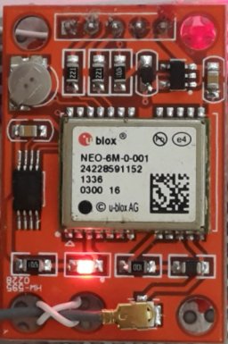
Fig 1.1 A Chinese board with the u-blox NEO-6M GPS module
Here I present two GPSDO designs. The first is a simple one, using a "classic" method, based on 1PPS pulses from a GPS receiver. It can work with any GPS receiver that provides a 1PPS output. It's performance is adequate, but not stellar. This was just a way of getting my feet wet in the GPSDO pond.
The second design does not use the 1PPS pulses, and only works with certain u-blox modules. (NEO-6M was used, but other 26MHz based ublox modules would probably work as well.) It requires a small modification on the ublox modules, but provides very good performance. This is achieved by using the sophisticated DSP inside the ublox chip to do the measurements, instead of trying to extract that data externally from the 1PPS pulses.
All of the measurements presented on this page are against a TEMEX LPFRS-01 rubidium controlled oscillator.
Up to table of contents
2. First version: KISS
Myself being more a slave than a domina, decided to try a gentler form of disciplining first, Keeping It Super Simple.
After a lot of web surfing about DIY GPSDOs, decided for a solution similar to the one
MIS42N (external link)
[1]
described on the EEVBLOG forum.
Basically, do almost everything in a microcontroller, using it's internal timers.
Unlike MIS42N, I decided to use a member of the MSP430 family, for no particular reason, except familiarity with the chips and tools. (And there is a breadboard friendly DIP version available.) I also decided to use the internal timer in a different way, as a kind of phase detector instead of as a frequency counter.
On the output I also use PWM, but instead of dithering, I use a dual step principle, like
Lars (external link)
[2]
, to get the resolution. It provides better resolution without reducing the PWM frequency, and unlike dithering, it does not introduce any frequency components below the fundamental PWM frequency.
2.1 PLL
The timer is run from the 10MHz OCXO, and set up to "capture" the 1PPS pulses. The timer's 16 bit counter will rollover many times during the one second interval, but the OCXO should be accurate enough itself, that the 1PPS will always fall into the same timer cycle.
If the OCXO's frequency would be an integer multiple of 65536Hz, one could simply let the timer count the full 65536 range. Then the captured value would directly represent the time error as a 2's complement value.
With a 10MHz OCXO, things are a bit more complicated. For example, the timer can be run with a 0...9999 cycle, for an 1kHz rollover frequency. The captured values are then from 0 to 9999, and one must "manually" convert the numbers from 5000 to 9999 to negative values from -5000 to -1, by subtracting 10000. The value obtained this way again directly represents the time error in 100ns steps, and the loop's task is to keep that at zero (or just constant at an arbitrary value, if all we need is a precise frequency).
Obviously, we have a 100ns dead zone, if we just work with the captured value.
No amount of averaging can help here, because the oscillator can stroll around within the 100ns window, and we will be totally oblivious about that.
A solution to this would be to make the loop stay on the switching point between two values..
In an ideal case, the loop would then constantly alternate between the two values, like a delta modulator encoding a constant value of 1/2, "sitting on the edge". A following (software) lowpass filter can reduce this dither to arbitrarily small values.
In practice, the "sawtooth" error on the 1PPS pulses will provide additional dithering.
2.2 FLL
Another possibility is to do a FLL loop. In this case, the difference between successive captures will be the loop error signal. With the OCXO exactly on frequency, the value read from the capture register will always be the same. When off frequency, the captured value will "drift". A difference of 1 (or -1) every 100 captures will represent a frequency error of 1E-9 (100ns drift every 100s).
2.3 Dual step PWM
This is simply two PWMs, connected together through a resistor circuit, so that at the output, the full range of the second PWM equals to one step of the first one. The second PWM thus provides a kind of "fractional step" capability to the first one.
How finely we can subdivide, depends on the accuracy of resistors and PWM output voltages. Coming from the same chip, and using higher value resistors, to minimize loading effects, it is probably safe to assume, that the PWM output voltages are matched quite well. So, with standard 1% resistors, the finest sensible subdivision would be bigger than 1/100. This assures that our scale will be monotonous, without "backsteps". 64 substeps will provide 6 bits of additional resolution. Choosing a power of two makes the arithmetic of separating the "coarse" and "fine" values in the software much simpler.
For the "coarse" PWM, we can use the capturing timer, which runs modulo 10000. This gives 13.2 bits of resolution. This uses up all of the capture timer's registers, so we need to use the other timer for the "fine" PWM. This also enables us to run the "fine" PWM modulo 64 at the internal 16MHz clock, giving it a frequency of 250 kHz. The internal 16MHz clock is just a RC oscillator, and will not be coherent with the 10MHz OCXO, but will "drift". Shouldn't be a problem, in any case, it could be avoided by running the second timer also from the 10MHz, for a 156.25kHz PWM frequency.
Potentially, this could cause a 250Hz beat with the 1kHz of the "coarse" PWM, but the high resistance in series with the "fine" output should take care of that. Also, 250Hz is still a much higher frequency, than what dithering by 64 would bring.
The two PWM outputs are combined with a 1:10000 resistor network, 1k and 10M, feeding a 560uF capacitor. This gives a 0.5 second time constant, which provides enough filtering of the slower, 1kHz coarse PWM, that any 1kHz sidelobes are below 80 dBc:
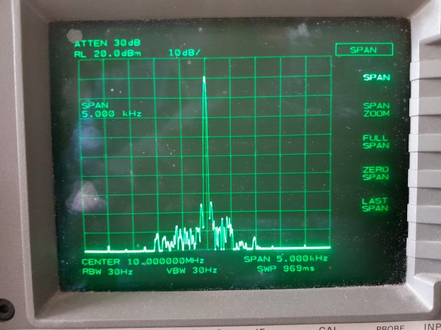
Fig 2.3.1 Output spectrum of an CTI OSC5A2B02 OCXO, controlled by a 1kHz PWM
Combined, we have 640000 steps (a little more than 19 bits) of resolution. At 3.3V, one step is about 5uV. Using a CTI OSC5A2B02 OCXO with 10Hz/V tuning sensitivity, one step equals to 50uHz, or a 5E-12 part in 10MHz.
The problem with PWM from a 3.3V microcontroller is, that the range of possible output voltages is only 0...3.3V. This is perfect for 3.3V oscillators, mostly OK for 5V types, but 12V oscillators might be a problem. Some have mechanical tuning, like the HP10811, which can solve this problem.
Up to table of contents
2.4 KISSDO v1
First, I made the simplest GPSDO I could think of. I used only the coarse PWM - one step is 3V/10000, which translates into 3mHz at 10Hz/V tuning slope of the CTI/CETC OSC5A2B02 OCXO.
This is 3E-10 relative at 10 MHz, fine enough for a 1E-9 accuracy, that I hoped to achieve with the KISSDO. Like, make all digits of an 8 digit frequency counter significant. This is the schematic:
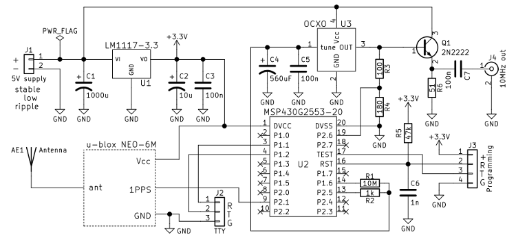
Fig 2.4.1 Schematic of KISSDO
The block labeled "u-blox NEO-6M" is not just the bare u-blox module, but the red Chinese board shown above.
There is no separate voltage regulation for the OCXO. This will of course come around and bite me (see below).
The microcontroller program has only a main function and a single interrupt function. The main function just sets all of the required peripheral registers for the timer and UART, and then enters an infinite loop, which outputs some data to the UART.
All of the disciplining is done in this ultra simple interrupt function, which implements a trivial FLL loop:
//convert captured value into signed time difference
if (TA1CCR1 < 5000) d=TA1CCR1; else d=TA1CCR1-10000;

//time derivative of time difference = frequency difference
dd = d - oldd;
oldd = d;
if (dd > 5000) dd-=10000;	//fix rollover
if (dd < -5000) dd+=10000;

//NOTE:  loop gain based on a 10Hz/V OCXO EFC
pwm = pwm - 32768*(long)dd;	//the loop Gain=0.5 => 32768
if (pwm < 5*65536) pwm=5*65536;	//keep within timer range
if (pwm > 9995*65536) pwm=9995*65536;

TA1CCR2 = pwm>>16;	//set PWM output
TA1CCR1 is the capturing register, and TA1CCR2 sets the PWM duty cycle.
The EFC value "pwm" is accumulated in an 32 bit variable (long), using a kind of "fixed point" arithmetic. The upper 16 bits represent the whole part, and are sent to the PWM. The lower 16 bits are the fractional part, allowing loop gains of less that 1. All other variables are 16 bit.
I was really very pleasantly surprised, how well it worked! Provided the OCXO is shielded from fast environmental changes (the CTI OCXO is quite small and low mass, so quite sensitive to air drafts etc.), it will hold within 1E-9. The 100ns dead zone proved to be much less of a problem, than what I feared it to be.
The down sides of KISSDO v1 are, that it needs hours to settle (depending on how far the OCXO was on power up), and that rogue pulses (the NEO 6M sometimes emits extra pulses anywhere between the regular 1PPS pulses) will badly throw it off, and it will again need a long time to settle.
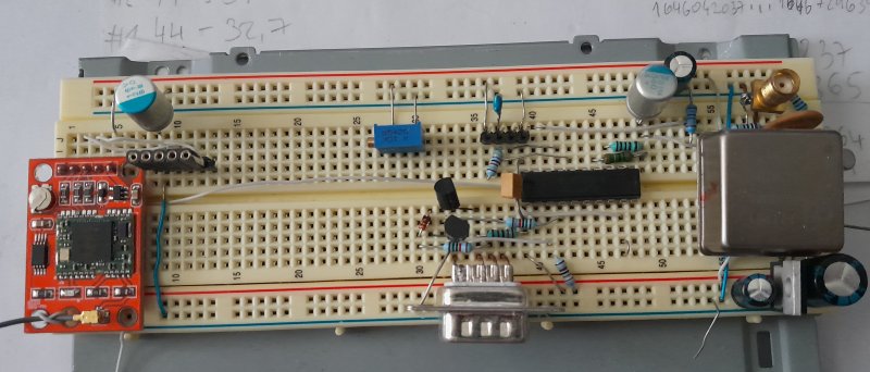
Fig 2.4.2 KISSDO built on a breadboard. The two transistors and resistors near the D9 connector are just for RS232 level shifting.
The five pin female header near te GPS board accepts an small USB/serial board, for communication with the Ublox.
A 100ns dead zone might seem to prevent us from getting more accurate than 1E-7 (1s/100ns = 1E7), so how can we avoid this? When the frequency is within +-1E-7, the captured value will mostly stay the same, only occasionally changing by plus or minus one. When these changes occur, we add or subtract a step to the EFC (PWM) value. If this step is small enough (smaller than the desired precision), the EFC will slowly be pushed toward the correct value.
The required smallness of the step causes the loop to be very slow. Besides the long settling time at start (and after rogue pulses) this also means it won't be able to track fast changes of the OCXO frequency. But with a reasonably stable OCXO, 1E-9 can be achieved using this scheme.
Up to table of contents
2.5 KISSDO v2
Same hardware, different firmware. To address the slow settling time, I wrote a slightly more complex disciplining function, which switches between three loop speeds, depending on how close the frequency is to the correct value. Also, when in the "closest" mode, it sets the step size based on the time passed from the last change in the captured value.
Apart from that, I added some code to try avoiding the rogue pulses. Quite ugly, a hodgepodge of counters and IF statements, I'm sure it could be done more elegantly, but it works.
Frequency deviations over a couple of days are shown below:
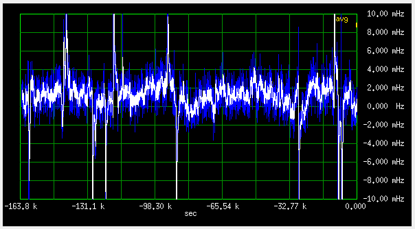
Fig 2.5.1 Frequency deviation plot of KISSDO v2
and are kept well within the +-1E-9 goal. Typically, it stays within a few parts in 1E-10.
Shorter term deviations look like this:
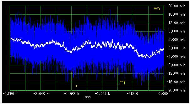
Fig 2.5.2 Short term frequency deviation plot of KISSDO v2
The non-averaged blue band is quite wide. I think the culprit is the 1PPS red LED blinking on the GPS board in combination with breadboard grounds and supply rails:
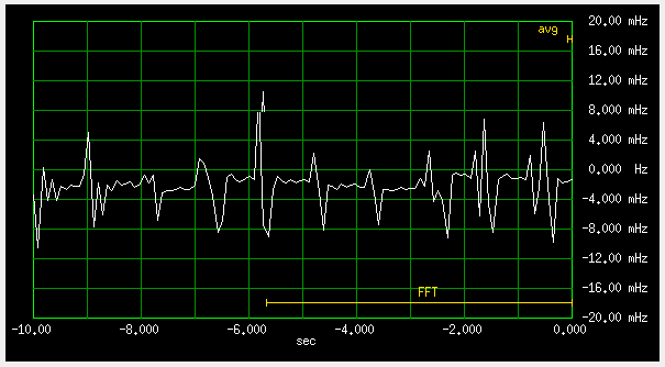
Fig 2.5.3 Blinking LED influences frequency
On a well designed PCB, with a separate regulator for the OCXO, these spikes should be absent.
I did not test these KISS designs very thoroughly, because this was not my intended final GPSDO solution, so it may contain bugs. I don't recommend either KISSDO v1 or v2 for "serious" use, these were just learning exercises for me.
The GPSDO rite of passage passed, it's now time to start a top notch GPSDO design!
Up to table of contents
3. Second version: A Message Based Self Disciplining loop
The MBSD is a further development of an idea proposed by
Simon Schroedle (external link)
[3] .
He proposed to use the u-blox NAV_CLOCK message, which reports the receiver's clock
offset, as the source of the error signal in the control loop, which can then control
the receiver's own clock oscillator. He also tested this in practice,
but did not develop it further.
To improve on this, I added a second loop, based on the TIM_TP-QERR message,
which has a much finer resolution, and makes a PLL possible.
I saw several advantages in this method, namely:
- it needs no hardware (external to, or inside the MCU) to measure 1PPS
- it bypasses the ublox internal hardware, which generates 1PPS (and other frequencies)
- it is inherently sawtooth-free
- it eliminates the (temperature dependent) delays of the internal/external hardware, etc.
Also, the external hardware has only one transition to measure each second, while the internal measurement can come directly from the code tracking loop.
The only down side is, that you have to do some surgery on the ublox module guts.
NOTE: later I found out that u-blox produces a self-disciplined module, the
LEA8F (external link)
[4] .
But looking at the
performance (external link)
[5] ,
I was not impressed, and decided to try to make a better, OCXO based MBSD GPSDO myself. (LEA8F can discipline an external oscillator, but in a somewhat complicated way, and the user has no access to the loop parameters.)
As a first step in this direction, I made a small program to draw some of the error parameters available from the QBX NAV-CLOCK, TIM-TP and NAV-DOP messages, to see how these behave.
The messages are sent by the ublox every second, so the horizontal scale on the graphs is one pixel per second, the whole horizontal span twelve and a half minutes.
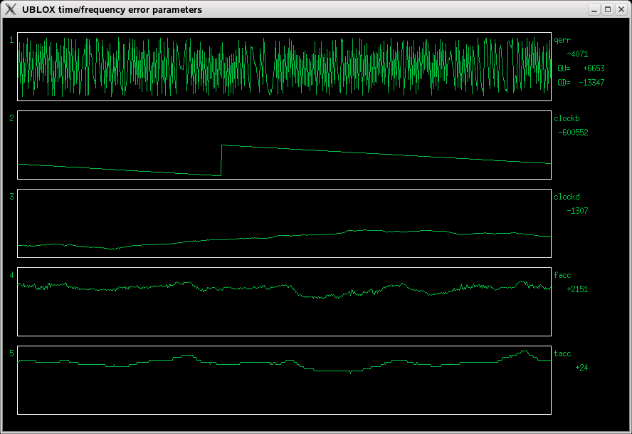
Fig 3.1 Typical error parameters plot of an unmodified NEO-6M
Graph 1 on the top, vertical scale -12000 to 12000, equal to +-12ns, shows that the
"sawtooth error" looks nothing like a sawtooth. Theoretically, with a constant clock
frequency offset, it would be a sawtooth, explaining the name. But as usual, real
world doesn't have much respect for theory. A simple xtal oscillator simply does
not have the stability, to keep the frequency offset constant enough.
To stay inside the same 26MHz clock period every second, the stability must be
better than 1/26MHz = 38.5E-9. With a frequency error of say, +-1E-6, the pulse
can fall anywhere within +-26 clock cycles from the "correct" value.
NOTE 12 dec 2023: Since other people seem to get a much nicer "sawtooth",
could it be that my ubloxes are fake Chinese, with ultra cheap oscillators? Bought them
off Ebay, of course :-) Otherwise, they seem to work OK.
The fact, that the reported value stays between +-10000 (+-10ns), seems to indicate that the 1PPS output pulses can be generated on both rising and falling edges of the 26MHz clock.
Every now and then, there is a slowdown in the "sawtooth error". That happens every time that the clock passes by a frequency, that has an integer number of cycles between pulses (an integer value of frequency in Hz). Ideally, that would be at 26E6 clock cycles between pulses, but it also happens at 26000001, 25999999, etc. clock cycles between pulses.
Next, I noticed that clockB (graph 2, second from top, scale -1.1E6...1.1E6) is just an accumulation of clockD, going to +-1E6 (+- 1ms) and then returning to zero. When receiving messages every second, this is redundant, as it can be easily calculated from clockD.
Graph 3 (mid, scale -1500...-1100) is the clockD (clock drift) value, a frequency offset with 1E-9 resolution. Seems quite well behaved, suitable as the input into a control loop for disciplining.
This is what Simon Schroedle used in his experiments.
Graphs four (second from bottom, scale 0...3000) and five (bottom, scale 0...30) show the fAcc and tAcc values from the NAV-DOP message. No idea what these measure - the Ublox receiver description only declares them to be "frequency accuracy estimate" and "time accuracy estimate", with no further description, or even equations.
They are unsigned values, probably the absolute value of something. In the above example, they seem quite correlated, but that isn't always so.
As they are called "accuracy estimates", does a higher number mean more accurate?
In fact, they seem more of an "error estimate", lower values being better.
To get some action into this movie, I controlled the room temperature by opening and closing the window (January...):
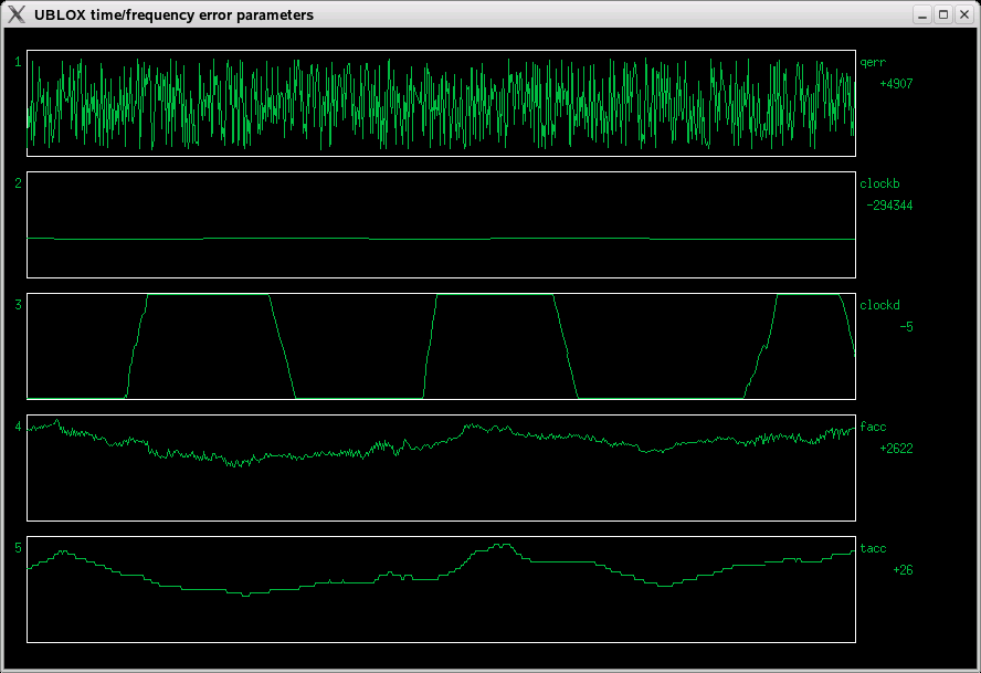
Fig 3.2 Forcing some change by periodically opening and closing the window
The temperature swing was a few degrees, and the clockD value varied between -2000 and +2000, maybe even more. The Ublox NEO-6M is a very high resolution thermometer, better than 0.01K resolution! The accuracy is of course questionable, probably depends highly on the accuracy of the supply voltage. Probably not very linear either, possibly even ambiguous with an AT cut crystal.
fAcc and tAcc show some motion, but really nothing that would reveal their true nature.
Next, I decided to replace the redundant clockB graph with the tdop (time dilution of precision) graph. This is a value which relates the time precision to the precision of pseudorange measurements, and depends mostly on satellite geometry. Ublox reports this value in the NAV-DOP messages, in percent (100 means a ratio of 1).
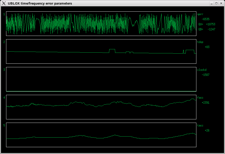
Fig 3.3 tdop instead of clockb
The jumps in the tdop graph probably happen when satellites are acquired or lost. The overall value is less than 1 (100), probably due to averaging between multiple sats.
These jumps MAYBE correlated with some humps on the fAcc/tAcc graphs - but on the other hand, the overall trend of tdop is down, while fAcc/tAcc go up on average! Still no idea what these represent...
Up to table of contents
3.1 External oscillator: TXEACDSANF-26
Time to try how this would work with an external clock oscillator. To open the NEO-6M module, I removed the sticker, and applied the biggest soldering iron at my disposal to the little tin box. It lifted nicely, just by the surface tension of the solder, no tweezers needed. This might seem a bit brutal, but when opening the first module, I tried a step-by-step approach with a smaller iron, and tore some copper off the tiny PCB. Luckily, these were just grounded pads for the tin box, and the module remained functional.
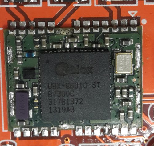
Fig 3.1.1 NEO-6M module with removed lid (note pulled off ground pad between the top pin rows)
To remove the crystal, I did not dare using hot air, not to blow away any of the 0201 components sitting around. So, I applied a somewhat smaller soldering iron to the top of the crystal package. At 350C it did not budge. So I cranked the iron up to 450C, and it released after a couple of seconds or so. The crystal is probably toast, but I lost the small sucker on the desktop/floor anyway.
I bought a Taitien TXEACDSANF-26.000 VCTCXO (Digikey 1664-1248-1-ND). First, I wanted to see how things work open loop, so I just connected the EFC (VCO) input to two potentiometers (coarse and fine regulation). Then I hooked the VCTCXO output to the Ublox, via a 150pF cap.
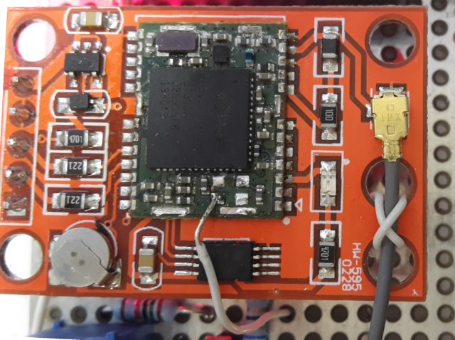
Fig 3.1.2 Clock directly coupled to former xtal pad
The ublox worked normally with this clock (regarding NMEA position data), but the error parameters ware quite horrible:
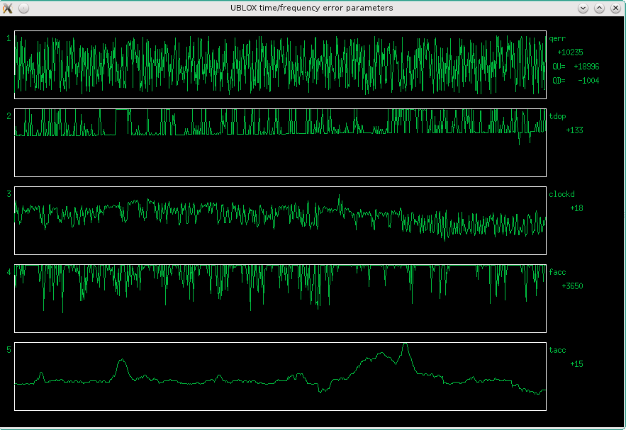
Fig 3.1.3 Error parameter plots with a direct coupled TXEACDSANF VCTCXO
Looks like this baby is quite picky about the clock! To improve things, I added a local LM1117 regulator and a bunch of additional RC filtering on both supply and EFC. Also two 15k resistors in series with the RXD and TXD serial lines. This did significantly improve the results, but the noise was still higher than with the original oscillator.
The small Chinese board with the ublox module has just a single ground pin, which now served for supply, serial port, and the 26MHz clock. This could bring some trash on the clock, especially the serial port. Therefore, I decided to transformer couple the clock. I found a couple of small (5mm od) ferrite rings in my junkbox. Together they had an Al of 250nH. Wound 11 turns of bifilar 0.3mm Cul wire. (Just kept winding until the hole was full.)
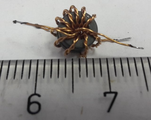
Fig 3.1.4 A small bifilar toroidal transformer for 26MHz
Since both VCTCXO and Ublox have DC offsets, I had to add 150pF capacitors on both sides.
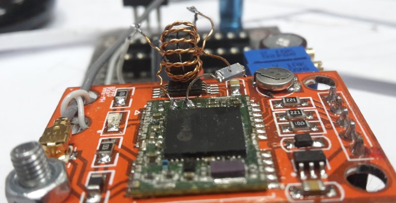
Fig 3.1.5 Installed transformer
Note the "air mounted" 1206 150pF cap. The whole thing now looked like this:
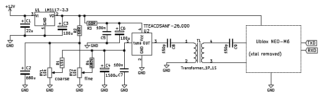
Fig 3.1.6 Schematic of external clock oscillator connection
Adding the transformer brought a slight further improvement, now things looked like this:
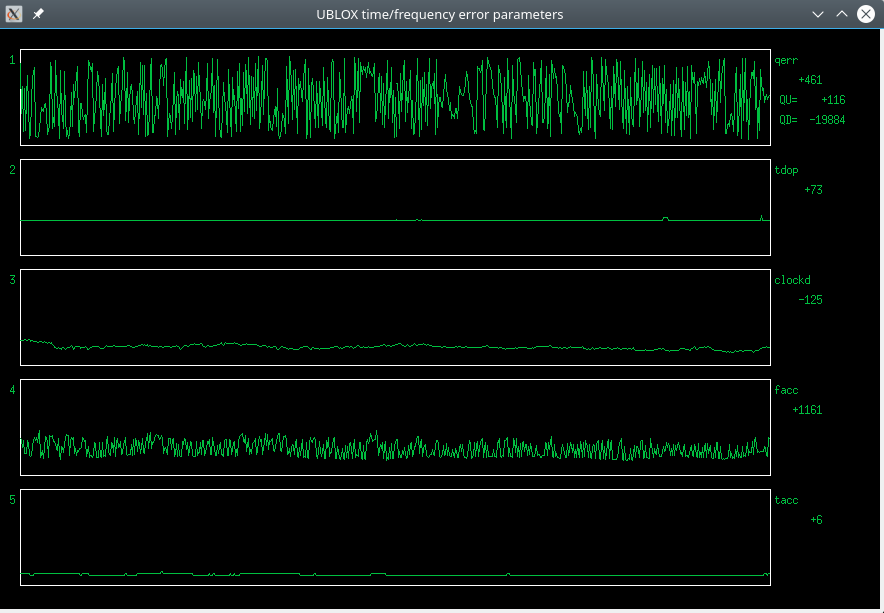
Fig 3.1.7 Error parameter plots with a transformer coupled TXEACDSANF VCTCXO
The overall longer term stability of clockD seems better, and the noise is gone from the tdop and tAcc graphs. Both tAcc and fAcc graphs are lower on average.
But there is still high noise on the fAcc graph. ClockD and the slow parts of qerr also seem noisier, compared to the original oscillator (compare with Fig 1 above). Whatever fAcc is measuring, it seems to be a sensitive indicator of oscillator noise!
To be sure, I connected another board that had the lid open, but still had the original oscillator, and repeated the measurement:
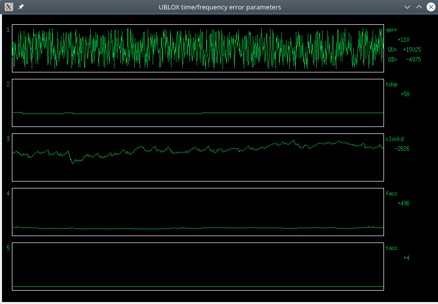
Fig 3.1.8 Error plots of another original NEO-6M
I did not open the window or do other thermodisturbing stuff. Despite that, clockD was all over the place, but fAcc was low and smooth?
FAcc is even smoother than the first NEO module with the original oscillator, before opening the lid!
I decided to check the phase noise of the TXEACDSANF VCTCXOs, one against the other. I made two small test boards:
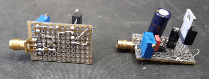
Fig 3.1.9 Two little protoboards with TXEACDSANF oscillators
They have a very weak (high impedance) output, so I had to insert a HP8447A amplifier, into both channels. Their tuning sensitivity is 200Hz/V.
The type is specified -145dBc/Hz at 10kHz, -135 at 1kHz and -115 at 100Hz, at 19.2MHz.
The result:
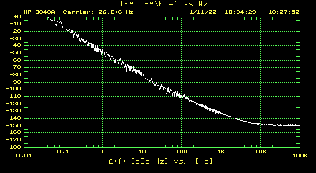
Fig 3.1.10 Phase noise plot of the TXEACDSANF oscillators
is within spec, considering this is combined noise of two oscillators, the amplifiers add some noise, and we must add 2.6dB (26 vs 19.2MHz). But clearly, nothing to write home about!
NOTE (8 feb 2022) It could be that some of the noise in the ublox measurements was caused by the low output level of the TXEACDSANF oscillators.
Up to table of contents
3.2 External oscillator: Telequarz TQOC 26
So, I decided to try getting something better. On Ebay, I found Tele Quarz Group type TQOC 26-01 26MHz OCXOs at a very attractive price. No datasheet to be found on the web, and a less round frequency probably contributed to the low price, so I bought five.
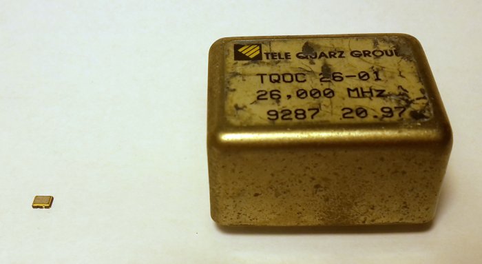
Fig 3.2.1 TeleQuarz OCXO (right), together with TXEACDSANF (left)
On the left is the TXEACDSANF VCTCXO. If size does matter, the TeleQuarz should really be better!
Having no datasheet, and the can having six pins, did not know how to wire it up. Ohmmeter brought no revelation, so I had to guess. One pin was clearly welded to the can, so this was ground. Next I tried 12V over a 100 ohm resistor to other pins, to see which will suck most current. No clear winner, but somehow I decided that the pin diagonally opposite to ground would be supply. Bingo, got 26MHz on another pin. Bottom view:
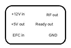
Fig 3.2.2 Pinout of the telequarz OCXO
The corner pins look like a mirror image (top view) of a DIP oscillator pinout. The can size is the same as the 10MHz Bliley, pinout is similar, except Bliley is a 5V type, has a 4V ref output, and no oven ready pin.
The telequarz starts to oscillate at about 6V, but to get the oven ready signal (after a few minutes at 24C), at least 7.5V is needed.
The output is a 5Vpp square CMOS waveform. Under 100ohm load it reduces to 3.3Vpp, and 2Vpp under 56ohm.
Tuning slope is about 7.5 Hz/V.
At 12V, cold it draws about 300mA, less than 100mA after 15min warm-up at 24C ambient.
Phase noise:
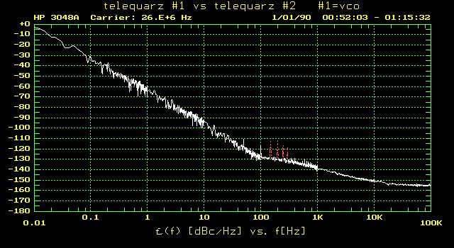
Fig 3.2.3 Phase noise plot of two telequarz OCXOs
at 100Hz and below is about 15dB better than the TXEACDSANF.
For the first test, I just put the OCXO "piggyback" on the protoboard:
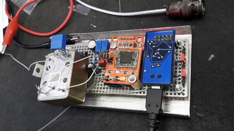
Fig 3.2.4 Telequarz OCXO piggyback on the protoboard
The blue board is just a serial to USB interface, to read the u-blox messages on a PC.
I was a bit skeptical about this makeshift construction, but
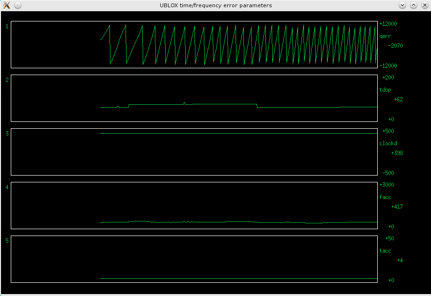
Fig 3.2.5 Error parameters with the Telequarz OCXO
Hooray!! Now we are talking! Check this out! Smoooooth!!!!
Even the quantization error looks now like it could cut some timber! The facc value is now quite docile too, but still no idea what it represents. So I decided to just ignore it from now on. Same for tacc.
Of course, next I manually tuned the OCXO to clockd = 0:
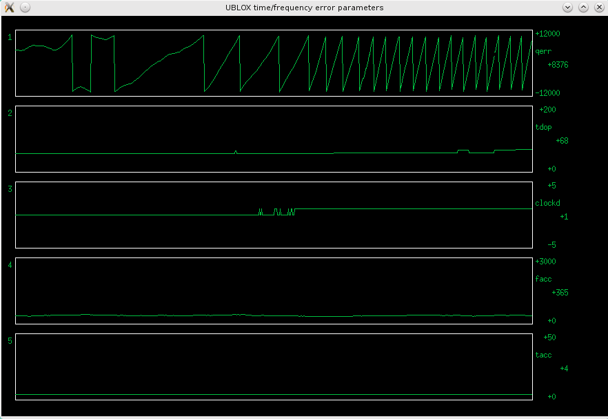
Fig 3.2.6 Error parameters with the Telequarz OCXO
The OCXO can be seen drifting to clockd = +1 over time. But we can also see that we have a similar (but smaller, 1ns vs 100ns) problem as in the KISS version above: a 1E-9 dead zone. (clockd is ns/s, a resolution of 1E-9.) We can see, on the quantization error, that the OCXO is wandering around, while clockd is zero all the time, until the OCXO drifts all the way to clockd = +1.
Unlike in the KISS PLL version above, we can't just sit between 0 and +1, which would introduce a fixed frequency offset of 5E-10, because clockD is a frequency, not a time measurement.
But then it dawned on me, that qerr is now tame enough, so we could probably make a "double loop", with the inner loop based on qerr, for fine control.
Qerr could not be used alone, because it is ambiguous, we can get a constant zero qerr at OCXO=26.000000MHz, but also at 26.000001MHz, 26.000002MHz, 25.999999MHz, (every 21 clockd steps) etc. So we need a "coarse" loop (based on clockD), that first brings clockd to zero, then we can switch to a "fine" loop, based on qerr.
Qerr is ps/s, a resolution of 1E-12. This is orders of magnitude better that any external measurement on the 1PPS pulses, it is ps versus ns - and we get such a precise measurement every second. With external 1PPS timing, one would need to average a huge number of pulses to approach this precision.
Of course, this is just the resolution. We are still subject to the GPS's intrinsic errors, like variable ionosphere delay, multipath, satellite clock offsets, satellite ephemeris errors, etc.
And, of course, the noise on the measurement will be much higher than a single picosecond, more likely in the hundreds of picoseconds (see below). Despite all that, we are still much better off, than with measuring the 1PPS output.
With a significantly reduced need for averaging, a much faster loop should be possible with qerr as the error input, maybe useful for less stable oscillators. But with an inferior oscillator, the qerr can become too scrambled to be of use, see the graphs at the beginning of this section. Also, one must watch out, not to spoil the short term stability of a good OCXO, with too fast a loop, like the
Trimble GPSDOs.
Keeping qerr close to zero also brings us "sawtooth free" 1PPS pulses, "for free".
Up to table of contents
3.3 The DAC problem
So, we can measure down to 1E-12. What would we need, to control the OCXO with the same resolution?
The 26MHz telequarz OCXO has a tuning slope of 7.5Hz/V. 26MHz times 1E-12 equals 26uHz, which corresponds to 3.5uV. Assuming a 5V full scale DAC, log2(5V/3.5uV) equals to 20.4 bits. So a 20bit DAC would just about cut it.
Wanting to design this one for high performance, I decided to go with a "real" DAC this time.
A nice 20bit DAC is MAX5719GSD, but it is quite an expensive chip (about 25 Euros). And it needs a precision external reference, which costs about the same. Well, I could use the 5V reference output of the telequarz OCXO, could be pretty stable, if it's inside the oven.
Browsing the distributor's sites, I found a whole bunch of cheap (5 Euros or even less) 24bit dual DACs available for audio applications. Of course, the first question is, can they output DC? And they use the quite non-microcontroller friendly I2S interface. And their internal reference is not very stable.
And they need their own clock (sigma-delta converters), which could cause interference.
But I soon ran into a totally different kind of problem: in the year 2022, we have a global chip shortage, and delivery times are measured in months. So this will have to wait, and I will have to stick with PWM for some time.
In the MBSD, we do not need to capture the 1PPS from the receiver, so we have one register left in the coarse PWM timer. To free the second timer for other purposes, like a software UART, we can use this free register to do fine PWM from the same timer as the coarse PWM. This timer runs modulo 10000, but wee need only 64 steps of fine PWM, so the fine PWM value needs to be multiplied by 10000/64 = 156.25. 0.25 is a nice binary value, so to keep all arithmetic integer, we can multiply by 4*156.25 = 625, then divide by 4.
3.4 First experiments
Since the place for the MSP on the protoboard was now occupied by the OCXO, I just hacked together the protoboard with the breadboard, on which I previously built the KISSDO:
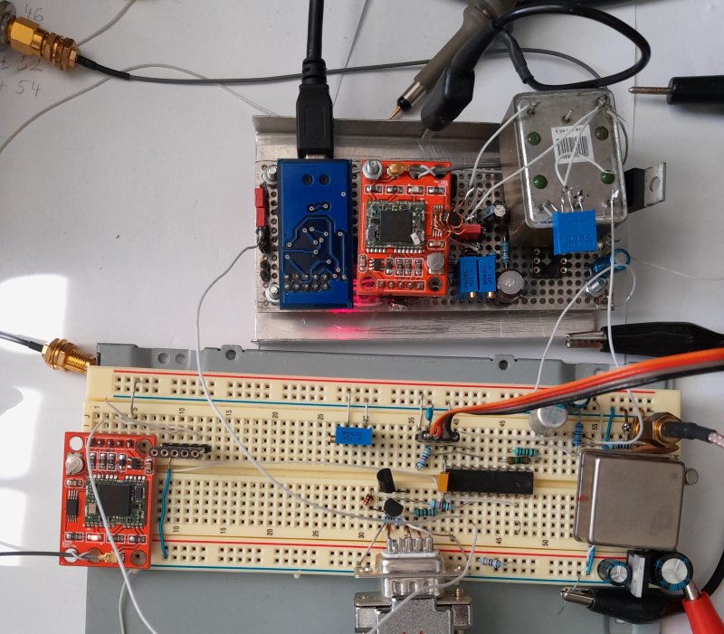
Fig 3.4.1 Protoboard and breadboard patched together
NOTE: The ublox and CTI OCXO on the breadboard are not in use here.
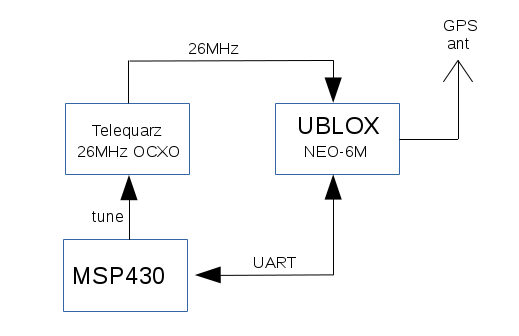
Fig 3.4.2 Block diagram of a simple MBSD loop
Despite the horrible hardware mess, after tuning the loops a bit,
this thing worked rather well. The following graphs show the behavior after resetting the microcontroller: (the ublox was already running and was locked to the satellites, and the OCXO had a couple of days to warm up before this)
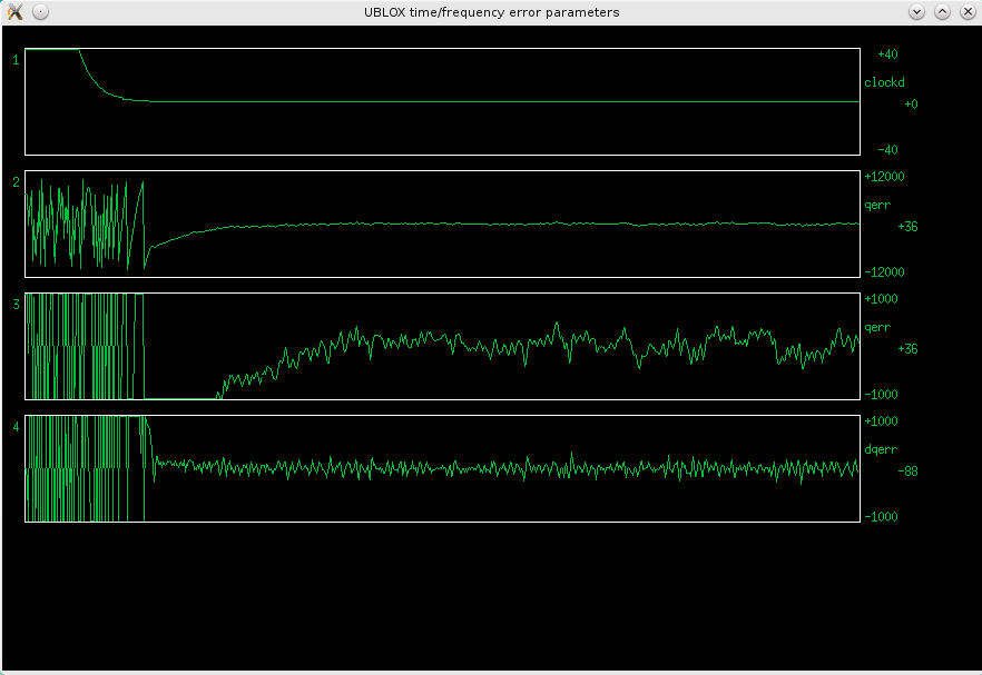
Fig 3.4.3 Error graphs of my first working MBSD. Time is scale one second per pixel, about 12 min the whole graph.
Note that I have changed the graphs a bit, #1 is now clockd, #2 is qerr, #3 is the same qerr, but on a magnified scale (+-1ns), and #4 is the difference between current and previous value of qerr.
On the top graph we can see how the coarse loop brings clockd to zero. Clockd then sits at zero and has no further influence on the OCXO control.
On the second graph from top, we can see qerr slowing down, as clockd goes below 3. When clockd goes to zero, a change in the slope of qerr can be seen, as the fine loop takes over, and pushes qerr toward zero.
Final accuracy is achieved in less than 5 minutes, and qerr is then held within +-500ps, not bad at all. The disciplining loop is again pretty simple: (most of the other code is just decoding the UBX messages)
int32_t dqerr;
int32_t maxqerr=18491;	//assuming max qerr = 0.5/26MHz [ps]
maxqerr=21000;		//for dqerr rollover fixing (empirical value)
//loop gains for telequarz OCXO, 7.5 Hz/v  @26MHz
int32_t clk_p=30000;	//clkd loop, proportional
int32_t qer_p=15;	//qerr loop, proportional	2...30
int32_t qer_d=600;	//qerr loop, differential	200...900

dqerr = qerr-oldqerr;
if (dqerr > (maxqerr>>1)) dqerr-=maxqerr; //rollover
if (dqerr < -(maxqerr>>1)) dqerr+=maxqerr;
oldqerr=qerr;

if (clkd !=0)	//coarse loop, clkd based
  {
  pwm -= clkd*clk_p;
  }
else		//fine loop, qerr based
  {
  pwm -= (qerr*qer_p + dqerr*qer_d);
  }

TA1CCR2 = (uint32_t)pwm>>16;			//coarse PWM
TA0CCR1 = ((uint32_t)pwm & briefcase) >> 10;	//fine PWM
This disciplining function is called each time both the NAV-CLOCK and TIM-TP messages
are received and decoded, which should happen once per second.
The rollover compensation is a bit inaccurate, because I haven't reliably determined
the maximum value of qerr. That is not a problem, because once the fine loop brings
qerr close to zero, rollovers won't happen.
The main function, after reset, sets up the MSR internal registers, then sends commands
to the u-blox, to switch it from NMEA to UBX protocol, and tells it which messages to
send, and how often. After that it busy waits for characters from the u-blox, decodes
the messages and calls the disciplining function.
The fine loop works well within a rather broad range of gain values, probably because we are in the flat valley between GPS and OCXO noise:
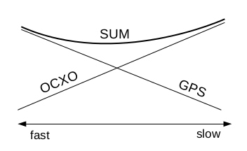
Fig 3.4.4 A graph of the sum of GPS and OCXO noises
The better the OCXO, the slower (lower gains) the loop should be.
The GPS noise here is probably mostly receiver noise and multipath, as the ionosphere and satellite errors are likely smaller at this time scale (they change slower).
Up to table of contents
3.5 26 to 10 or 10 to 26?
A problem with this MBSD is, that we now have a 26MHz disciplined oscillator, but most
applications require a 10MHz reference. If not for other reasons, to compare this to
other 10MHz standards, I needed to do something.
I could think of three possibilities to obtain 10MHz:
- Make 10 MHz from 26 MHz, for example with a PLL
- Use the MBSD to discipline a 10MHz OCXO, then make 26MHz for the receiver from this
- Use the now "quasi perfect" 1PPS pulses to drive a "classic" GPSDO
Because 10MHz OCXOs are more widely available, I choose the second option. Also because
the HP10811 OCXOs were much better than the 26MHz ones I had.
Nonetheless, I decided to design something that would support both options 1 and 2, using a simple PLL synth chip from Analog Devices, the ADF4002. These only come in tiny SMD packages, so I had to design a PCB. To program the ADF4002, I added a small MSP microcontroller onto the board. For the VCXO, I designed a footprint, that should accept most four pin SMD oscillator packages. This is the schematic:
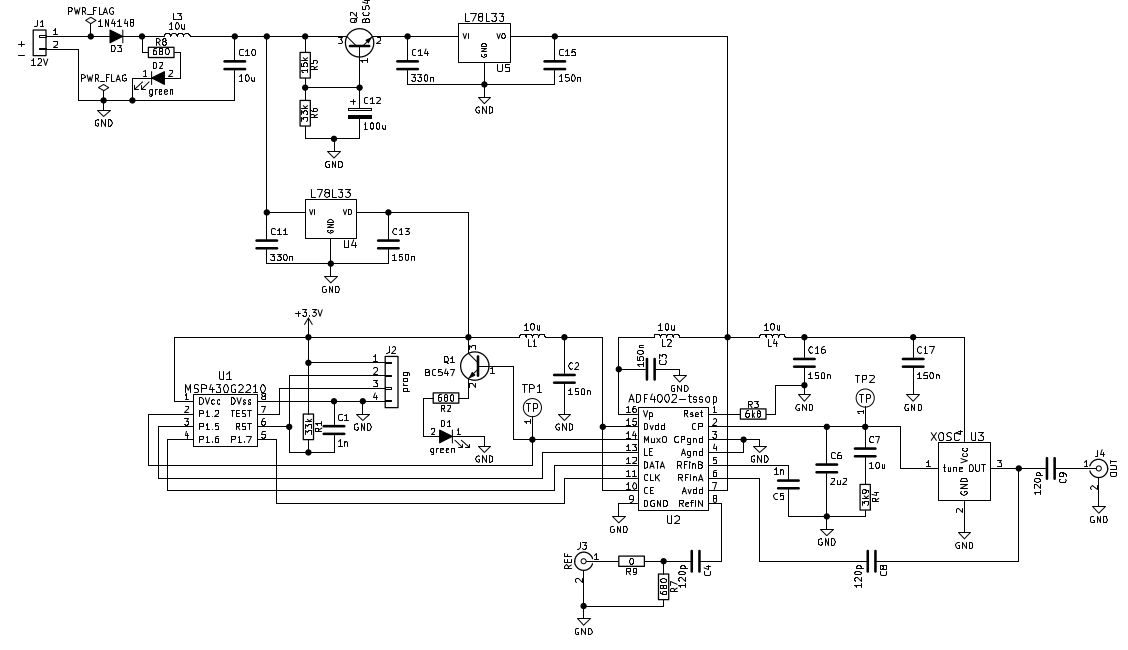
Fig 3.5.1 Schematic of the 26 to 10MHz (or vice versa) VCXO synth
When phase locking a crystal oscillator, one usually wants to make the loop very slow,
to let the crystal show it's virtues. But here, the HP10811 I intended to use as the
disciplined 10MHz source, has a phase noise more than 40dB lower than the TXEACDSANF,
for offsets below one hertz. So, a wider loop should be beneficial. In an integer synth,
the highest possible phase detector frequency, that divides both the 10MHz reference
and the 26MHz output, is 2MHz. That would easily support a 100kHz wide loop.
But for a simple RC loop filter and 100kHz loop bandwith, ADI SimPLL spat out
impractically low values for the filter capacitors. Not wanting to introduce
noisy opamps into the loop, the only solution was to squeeze the loop bandwidth.
At 10kHz loop BW, C6 was still only 8.2 pf, comparable with PCB trace capacitances
and TXEACDSNAF input capacitance (not specified in the datasheet, but probably in
this ballpark). Squeezing further down to 3.15kHz, finally gave reasonable 82pF
and 390pF capacitors, and R4=330kohm.
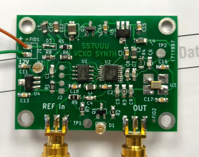
Fig 3.5.2 The 10 to 26 or 26 to 10 MHz PLL board
The ADF4002 ref input, for sinewaves, is specified only down to 20MHz. I tried with a 1.5Vpp sine, and it divided down to about 3MHz input. Feeding it a square wave from a HP33120, it worked down to 100kHz. With a steeper square, like from an 74HC gate, it would maybe work even further down.
With a 10MHz sine, it worked down to 0.3Vpp (specified sensitivity at 20MHz is 0.8V), so we have a lot of spare room, driving it with a 10 MHz sine.
To get some mechanical stability, I just bolted everything onto a random piece of aluminium.
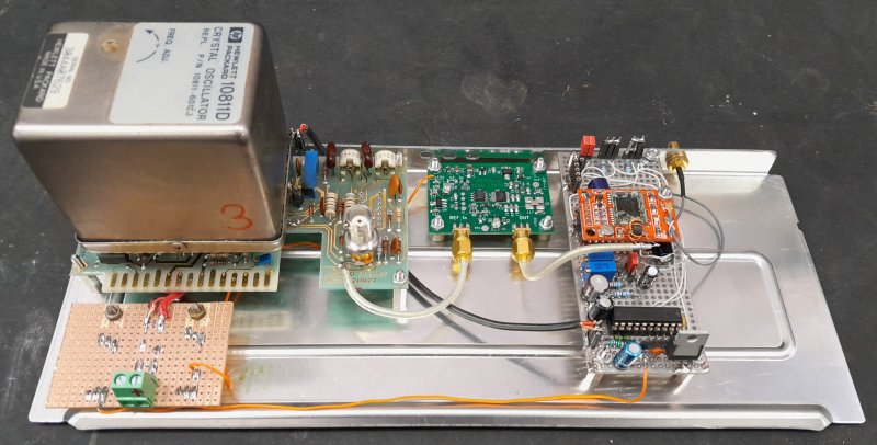
Fig 3.5.3 All of the stuff mounted on a chassis
The stripboard on the left hosts a 7805 and a 7812, so that the whole contraption runs from a single 20...24V supply (needed for HP10811).
This is the block diagram:
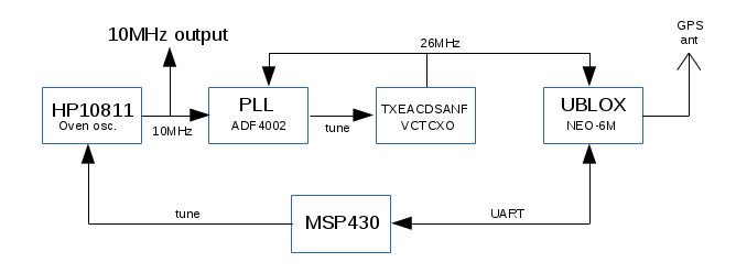
Fig 3.5.4 Block diagram of the 10MHz MBSD
But the output of the TXEACDSANF was too low to reliably drive the ublox, so I had to add a simple AC00 based 26Mhz buffer:
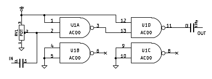
Fig 3.5.5 Schematic of a 26MHz buffer with 74AC00
A HC00 would probably also work. The 26MHz from the TXEACDSANF is just a couple hundred mV p-p, so the adjustment of RV1 is very critical. Did not use the "feedback bias", because in the past, encountered some stability problems with AC logic in that configuration.
The AC00 outputs 5Vpp, which could be dangerous for the 3.3V ublox, but the "short" transformer described above, reduces (by loading) the amplitude to about 2Vpp.
In the final solution, I'll use an analog amplifier.
Up to table of contents
3.6 Tuning the loops
There are two loops in the MBSD firmware, one based on the "clockd" value from the NAV-CLK message, and one based on the "qerr" value from the "TIM-TP" message.
The ADF4002 hardware PLL has a fixed bandwidth of 3kHz, which is orders of magnitude faster, and needs not be considered, when tuning the MBSD loops.
Also, the 0.5 second RC constant in the PWM, can in most cases be ignored.
The "clockd" loop only has a proportional channel. Since "clockd" represents a frequency offset, this is a FLL loop. It is a first order loop, having only a single parameter, so it is easy to tune. It is used as a "coarse" loop after reset, to tune the OCXO to within 1E-9 (the resolution of "clockd" is 1ns per s), then it remains inactive as long as the OCXO remains within 1E-9 - which it should always do, unless there is something wrong, like a totally out of tune "qerr" loop. Therefore, it does not influence the final accuracy of the MBSD, and the gain can be set quite high (like clk_p=1000000), for fast action.
The "qerr" loop has proportional and differential channels. No integral channel, because VCOs have no friction. Since "qerr" represents a time offset, the proportional part is a PLL, and the differential part is a FLL. The "qerr" loop is used as a "fine" loop, to precisely tune the OCXO.
The loops are tuned by changing the values of variables in the MSP firmware, function discipline(). The "clk_p" variable is the gain of the "clockd" loop. The variables "qer_p" and "qer_d" are the gains of the proportional (PLL) and differential (FLL) parts of the "qerr" loop. The "qer_p" mostly sets the loop's own frequency, and "qer_d" mostly sets the damping of the loop.
After each change of the gains, one has to wait from minutes to hours, for the loops to stabilize, and then some more, to observe the behavior. Tuning a slow loop can take days!
The "clockd" loop can be tuned by resetting the microcontroller and watching the "clockd" value. The loop should quickly, but without overshoot and oscillation, bring "clockd" to zero.
On the other hand, tuning the "qerr" loop for minimum "qerr" deviation does not give optimal results, as described below. This loop should be tuned using an "real time frequency comparator", something like my
FRCOMP,
and a stable reference (a free running good OCXO, or a rubidium or other atomic standard).
3.6.1 Fast loop
After changing OCXO from Telequarz 26Mhz to the HP 10MHz, which has a much lower tuning slope, I had to re-tune the loops. By tuning for minimum "qerr" deviation, I could easily reproduce the results from earlier:
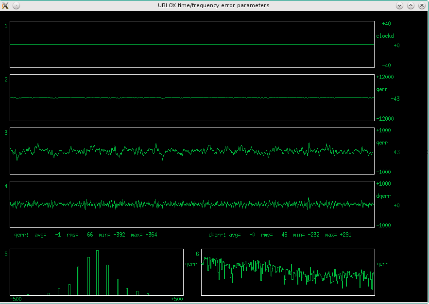
Fig 3.6.1.1 Error plots with the MBSD tuned for minimum qerr deviation (qer_p=-19000 qer_d=-200000)
When the HP10811 holds the TXEACDSANF tightly by the throat, it seems to be quiet enough for the ublox!
I have again changed the program, so it now draws a histogram (from -500 to 500 ps in 10 ps steps) and spectrogram (512 point real FFT at 1sps) of the qerr. The histogram looks quite "Gaussy", and there are no suspicious humps in the spectrogram, so far so good.
Note the "comblike" histogram - the resolution of "qerr" seems to be much coarser than 1ps! Looking closer, between -100 and +100 ps, I could only see the values [-100,-41,+16,+74]. But on other occasions, they were [-103,-45,+13,+71] or [-86,-28,+29,+87], [-57,0,+58], etc. So the step size looks to be between 57 and 59, however not always on the same steps.
But now I had a 10MHz output on the MBSD, so I could compare it with a lpfrs rubidium:
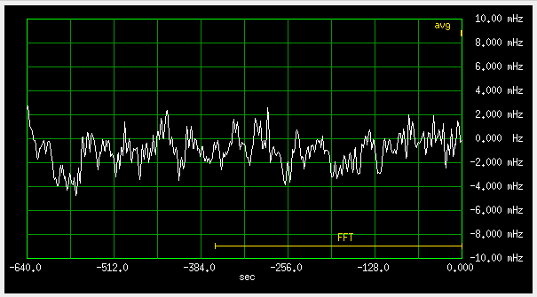
Fig 3.6.1.2 Frequency deviation, fast loop (qer_p=-19000 qer_d=-200000), 2mHz/div
OUCH!!!
This is really bad, especially considering that a free running HP10811, compared to the same rubidium, at the same scale, looks like this:
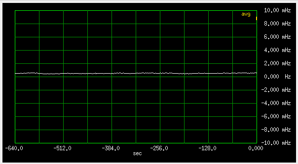
Fig 3.6.1.3 Frequency deviation, free running HP10811, 2mHz/div
The jumping is similar to the
TRIMBLE
GPSDO. The Trimble uses a D/A chip, so the jumps are quicker than my PWM with a big RC constant, but otherwise, a strong family resemblance can be observed. Looks like the Trimble uses a similar disciplining method, with similar loop parameters.
Obviously, tuning the loop for minimum "qerr" deviation makes for a fast loop, that faithfully follows the noise in the GPS receiver. On the positive side, it achieves the initial lock quickly (a couple of minutes), and long term average accuracy will be similar to a slower loop.
But, as stated at the top, I also need short term stability and low phase noise.
Up to table of contents
3.6.2 Slow loop
To avoid spoiling the short term stability of the OCXO, a much slower loop is needed.
So I reduced the "qerr" differential loop gain by a factor of 600, and set the
proportional gain to zero (a pure FLL). Such a slow loop requires a top-notch OCXO.
With my best HP10811 (#3), I got these results:
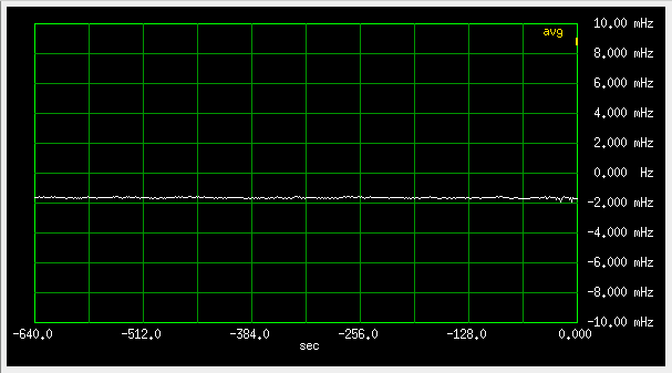
Fig 3.6.2.1 Frequency deviation, slow loop (qer_p=0, qer_d=-32), 2mHz/div
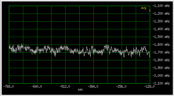
Fig 3.6.2.2 Frequency deviation, slow loop (qer_p=0, qer_d=-32), 100uHz/div
which is pretty good. The -1.7 mHz offset is of the rubidium.
Letting it run over the weekend, nobody home, gave this result:
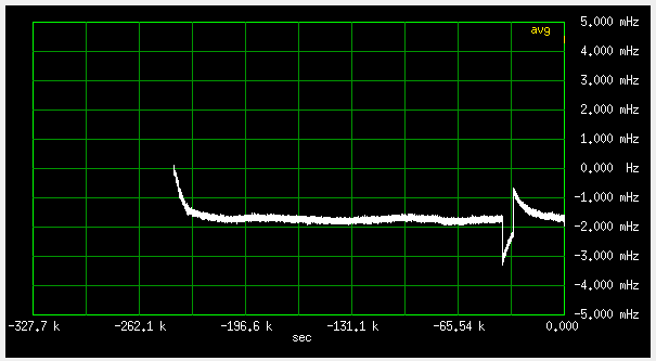
Fig 3.6.2.3 Frequency deviation, slow loop (qer_p=0, qer_d=-32), 1mHz/div
On the left is the startup transient, followed by two days of steady state, and then a strange event at right.
The initial transient is MBSD loop only (microcontroller reset), OCXO and GPS were already running and stable.
In the steady state, expanding the vertical scale:
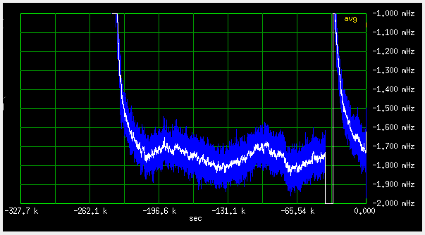
Fig 3.6.2.4 Frequency deviation, slow loop (qer_p=0, qer_d=-32), 100uHz/div
the short term (blue) deviations are about 100uHz (1E-11) peak, probably mostly from the rubidium phase noise. A couple of 24h diurnal cycles can clearly be seen. The difference between day and night is about 100uHz (1E-11). This is either due to room temperature, or GPS ionospheric effects. The temperature during the measurement is shown in the graph below:
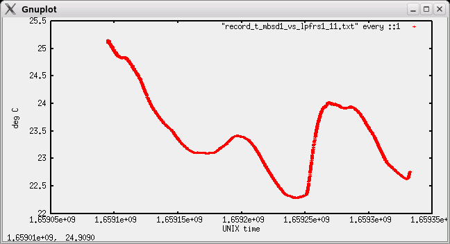
Fig 3.6.2.5 Room temperature variations during measurement
The temperature could affect either the rubidium, or the OCXO, with the loop to slow, to regulate it out. I did some testing on the rubidiums, and their thermal constant is too small to cause such deviation. So the 24h variation is either loop too slow, or ionosphere.
The strange event to the right, expanded, looks like this:
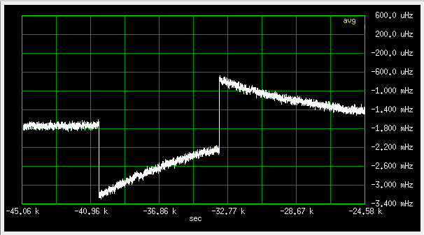
Fig 3.6.2.6 A strange event during measurement, slow loop (qer_p=0, qer_d=-32), 400uHz/div
It happened on Sunday, between 6 and 10 in the morning, when nobody was around.
Looks like somebody injected a 4h long, 1.5mHz square pulse into the loop.
No idea what that could be. A bug in the MBSD firmware? A hiccup in the ublox?
The jump size is about one step of the clockd loop at clk_p=1000000, so I guess
clockd woke up for some reason, known only to ublox. Normally, clockd should be
zero for frequency errors less than 5E-10 (5mHz at 10MHz).
Later I found out, that the OCXO does these jumps, for a few days, after it has been
powered up.
The loop time constant can be estimated from the transients, to be about two hours.
To check, how often this happens, I did another record, over about 3.7 days:
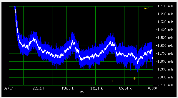
Fig 3.6.2.7 Frequency deviation, slow loop (qer_p=0, qer_d=-32), 100uHz/div
On the left is the switch-on transient. The 24h cycle can clearly be seen.
No jumps this time!
The temperature went like this:
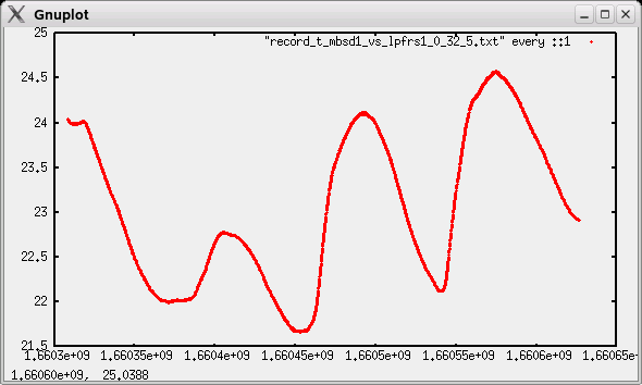
Fig 3.6.2.8 Temperature plot
There is an overall down trend in frequency, and up trend in temperature, so there might be some causal connection. Can't really say whether this is the rubidium or the MBSD, I have reached the limits of my indie lab here.
This time I also recorded the GPS spatial coordinates. Height has the most pronounced 24h cycle:
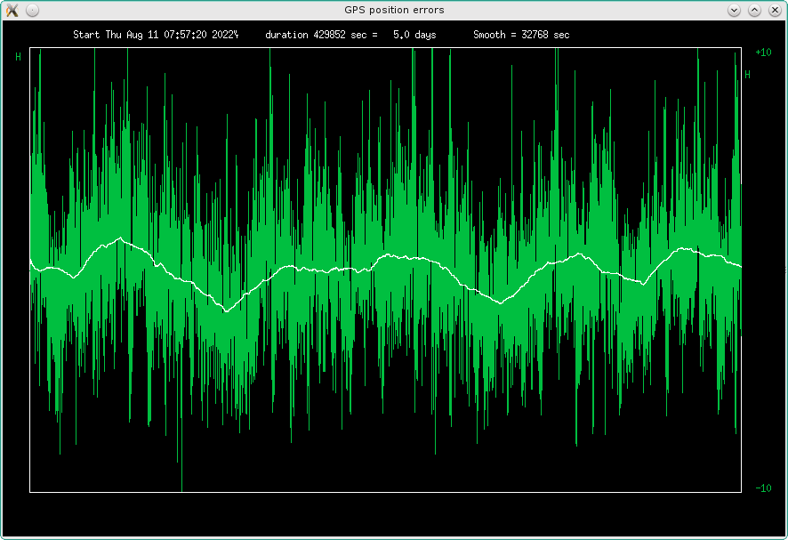
Fig 3.6.2.9 Plot of GPS height coordinate, vertical range +-10m
The GPS record started about a day earlier, so ignore the leftmost part of the plot. The daily deviation in height is about plus minus one meter. This would correspond to about plus minus three nanoseconds. A 24h sinewave of this amplitude would have a maximum slope of 7.3E-14. The height is not a sinewave, it has some steeper parts, but I guess the frequency errors should still be below 1E-12. Of course, they will depend on solar activity, so the worst case errors could be much higher during a big solar fart.
During this recording (12 Aug...16 Aug), this was the Sun's activity:
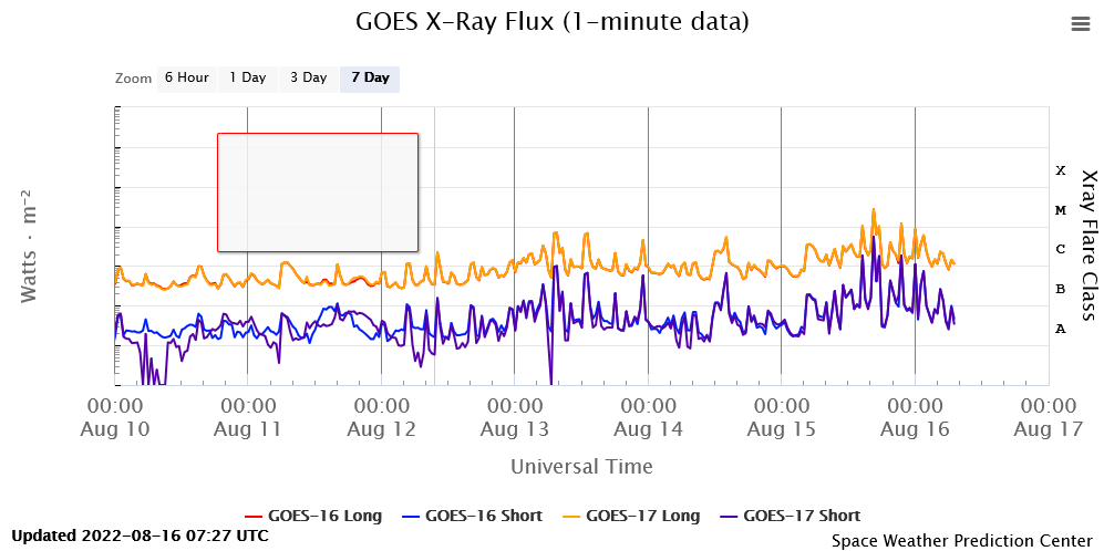
Fig 3.6.2.10 Plot of Solar xray flux (from https://www.swpc.noaa.gov/)
Setting "qer_p" to zero, the "qerr" loop becomes a first order loop, with a nice exponential response. But this also means that the phase (time) is not regulated, and can drift. So, strictly speaking, with this tuning, the MBSD is an accurate frequency reference only, not providing absolute time.
With this slow loop (qer_p=0, qer_d=-32), "qerr" now behaves like this:
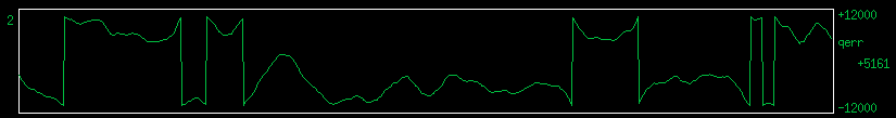
Fig 3.6.2.11 "qerr" from ublox, slow loop (qer_p=0, qer_d=-32)
The wiggles above are almost exclusively due to the GPS receiver.
The loop is now quite slow, it can take many hours from start to settling down. A solution for this would be, to start with a higher gain, and later decrease it, as the loop settles down.
Another drawback is, that it can not regulate out fast changes of the OCXO, like a wind gust hitting it, or an abrupt supply voltage change. Therefore, this slow loop MBSD should be put into a (massive) box, with good supply voltage regulation.
Up to table of contents
3.6.3 Medium loop
To get phase (time) under control, we must use "qer_p". Theoretically, we could do a first order PLL by setting
pwm = qer_p * uqerr;
but in practice this does not work, because in the beginning, the frequency is far off, and "qerr" is too fast for unrolling to work (see below). We can't use the "clockd" trick, because when we switch to pwm=qer_p*uqerr, any previous value of pwm is forgotten, and it starts from scratch.
Therefore, we use the same
pwm -= (uqerr*qer_p + dqerr*qer_d);
loop as before, in the fast loop.
This loop is of second order, and can do some swinging and dancing. Using "qer_p" alone, gives a differential equation with only the second derivation, whose characteristic polynomial, for negative qer_p, has roots on the imaginary axis: zero damping, swinging into eternity. For positive qer_p, roots are on the real axis, but one is positive, booom!
To keep that under control, the damping (qer_d) must be increased significantly. But differential channels are famous for noise amplification (see the fast loop above), so we must strike a balance between swingy behavior and noise intrusion.
With "qer_p" not zero, there is another problem we must solve: "qerr" from the ublox is ambiguous (cyclic, "modulo"). When it reaches about 10ns, it "rolls over", to about -10ns, causing a reversal in the loop. With the fast loop, "qerr" was kept below a nanosecond, so no rollovers happened, and this was not a problem.
But with slow loops, it can wander beyond 10ns, causing rollover problems. It is not hard to "unroll" it in the software, but that leads to another problem. After reset, frequency is off for some time, and the "unrolled qerr" will accumulate a large value. The slow PLL will then take a lot of time, to bring that down. During that time, it must push the frequency off, to move "unrolled qerr" from far away back to zero.
The solution I used was to force the "unrolled qerr" to equal "qerr", while "clockd" is nonzero ("clockd" loop is active), to reduce the windup.
While trying to unroll "qerr", I noticed another strange thing. With a 26MHz clock, both flanks active, one would expect a maximum quantization error of +-0.25/26MHz, that is +-9.615 ns. But "qerr" goes beyond +-10.5 ns. The only explanation, that I can think of, is that the guys at ublox added some 1000 counts of hysteresis, to keep "qerr" from wildly jumping.
NOTE: 10.5ns looks like a 48MHz clock, as some other Ublox chips use, but there was no such clock around here!
After some playing with the gains, qer_p=-2 and qer_d=-415 seemed to be a good tradeoff:
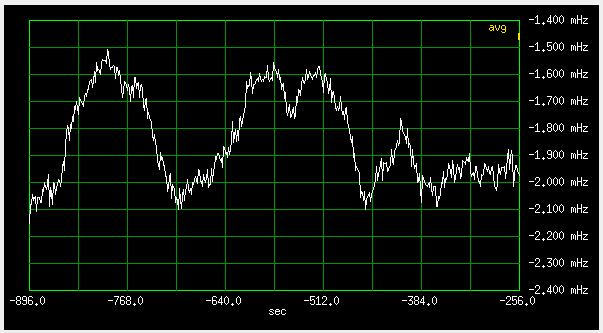
Fig 3.6.3.1 Frequency deviation, medium loop (qer_p=-2, qer_d=-415), short time, 100uHz/div
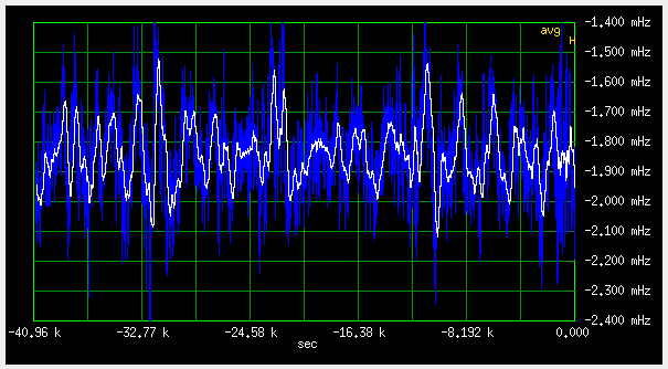
Fig 3.6.3.2 Frequency deviation, medium loop (qer_p=-2, qer_d=-415), longer time, 100uHz/div
I'm a bit uncomfortable with such low number for qer_p, it means coarse control, and would prevent having the same gain with a steeper tuning OCXO. I guess, in the final version of the firmware, I'll use a 64 bit accumulator. The loop calculation is only done once per second (ublox message rate), so the microcontroller could easily do float. But a standard 4 byte float has only 24 bits of mantisa, so it would be even worse than a 32 bit integer.
Up to table of contents
3.6.4 Different OCXO
Calculating the loop gains for a different OCXO is simple: just multiply the gains by the ratio of tuning slopes. For example, switching from the HP with -0.3Hz/V to an Epson with +1Hz/V, multiply the gains with -0.3 (higher slope needs less gain, note also inverted sign).
Besides the slope, the quality (stability) of the OCXO must be considered. A better OCXO can run with a slower loop (smaller gains).
One problem, when using other OCXOs, can be the small 0...3.3V output voltage range of the PWM. With HP10811, it's mechanical tuning option can solve this.
3.6.7 Comparing the loops
Comparing the three loop tunings described above, none is "simply the best". One must decide, which one suits the problem at hand best. The difference is mostly in the short term stability. The long term stability is determined by GPS errors, and should be the same among the three loops.
The fast loop.
This one is good, if fast locking is desired. It seems that the commercial telecoms type GPSDOs are tuned this way.
Short time frequency deviations will be much higher than with the slower loops, but the long term average will be the same, since it is determined by the GPS signal itself.
The same is true for time deviations.
The advantage is fast locking, the start up time being mostly determined by oven warm up.
The medium loop.
This one is a trade off between short time frequency stability and time accuracy.
Short time frequency stability will be better than with the fast loop, but worse than with the slow loop.
Short time timepulse accuracy will be better than the fast loop, because the OCXO will smooth out some of the GPS wobble.
The slow loop.
Provided you have a very good OCXO, this one is designed for best short term frequency
stability. Time is not locked, and can wander away.
It is the best option, if you just need a low noise frequency reference.
It needs hours to days, to stabilize after power up.
It is not an instrument, that could be powered up "on demand", it should run 24/365.
Up to table of contents
3.7 Testing, round 1: antenna positions, signal level
Having a working example, I could start some testing, planing to do more testing later,
with the final version, built on a single PCB. I was mostly interested in the short term
stability, since the long term stability will be that of the GPS system, provided the
loops keep tracking.
Later, when I have a couple of MBSDs, I will compare the outputs of two identical loops,
connected to the same antenna, like I did with the
Trimble GPSDOs.
This will eliminate the GPS system errors, and only show the performance of the
receiver DSP and GPSDO loops. Even the noise will be mostly the same in both
receivers, as it comes mostly from the antenna.
To check the effect of noise, the two receivers could then be run from separate antennas.
3.7.1 Antenna position
I decided to test the influence of antenna positioning, by comparing the frequency deviations with three different antenna positions:
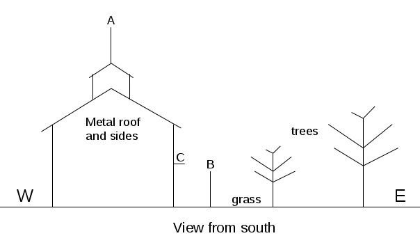
Fig 3.7.1.1 Antenna positions A, B and C.
The blasphemous idea of using an indoor antenna, didn't even come to my mind.
At position "A", there was the antenna, that came with the Oscilloquarz GPSDO, a small white dome. At positions "B" and "C", there was a small black square "puck" antenna from Ebay (the same one, moved between between the two positions). Obviously, this is not really a fair comparison, since one antenna is of different type, but I'm slowly getting too old for roof climbing.
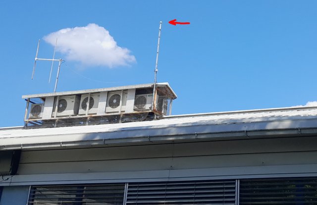
Fig 3.7.1.2 Antenna "A".
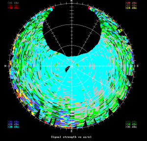
Fig 3.7.1.3 Heather signal versus angle plot of antenna "A".
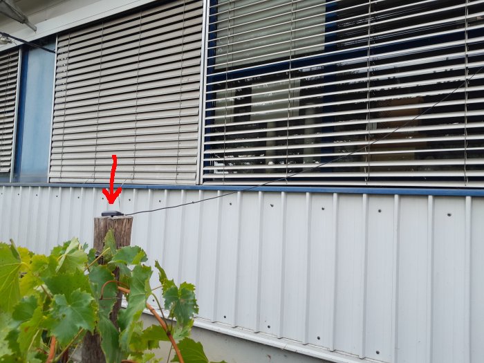
Fig 3.7.1.4 Antenna "B".
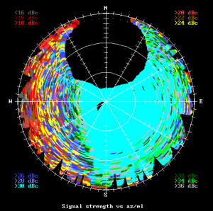
Fig 3.7.1.5 Heather signal versus angle plot of antenna "B".
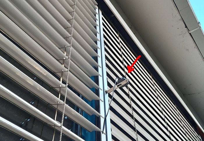
Fig 3.7.1.6 Antenna "C".
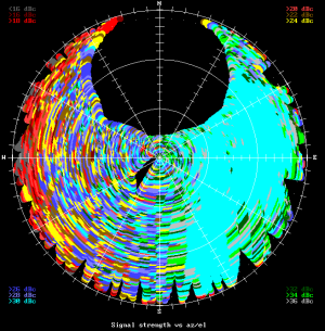
Fig 3.7.1.7 Heather signal versus angle plot of antenna "C".
Not sure how antenna "C" can see anything in the western sky? I guess reflections from the trees - but they don't help much, as can be seen from the results below.
In the beginning, I was using only antenna "A" for all experiments. The signal was a bit lower, because of the long cable, but otherwise it seemed ideal, having an unobstructed view of the sky.
But then I started to notice some periodic disturbances in the loop, maybe these were due to multipath (ground reflection). The antenna "A" being quite high, it could "see" a lot of ground in the sidelobes, and the metal roof could also contribute.
Here is a typical example:
Watching the "qerr" graph (like watching grass growing :-), once I noticed a strange behavior, a periodic component suddenly appearing:
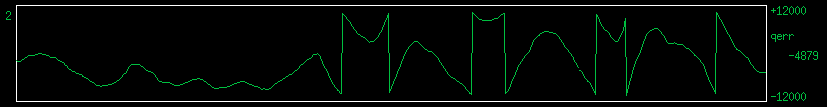
Fig 3.7.1.8 "qerr" from ublox, slow loop (qer_p=0, qer_d=-32), antenna "A"
the period being about 130 seconds. A few minutes later, it disappeared as swiftly:
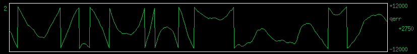
Fig 3.7.1.9 "qerr" from ublox, slow loop (qer_p=0, qer_d=-32), antenna "A"
Just before it disappeared, it reached an amplitude of 65ns pp, and the loop, albeit slow, was starting to track it:
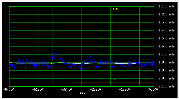
Fig 3.7.1.10 Frequency deviation, slow loop (qer_p=0, qer_d=-32), antenna "A"
causing a 100uHz (1E-11) deviation.
So, what was this?
Could it be ground reflection? For a 130 second period, the difference between direct and ground reflected path should change by one wavelength in 130 seconds, about 1.5mm per second. For a 12h orbit and my approx. 10m high antenna, this happens at about 62 degrees elevation. So, we are in the ballpark - but the quick appearance and disappearance seem a bit odd, and one would expect ground reflections at lower elevations, where reflection is stronger because of shallower angle, and antenna sidelobe pattern is higher. So maybe it was not ground, but some QRM, or a low flying airplane? I forgot to check the next day, if the same happened four minutes earlier.
To check this, I used the other two antennas. The fast loop should track the wiggles, making them visible on the frequency deviation graph. The graphs were plotted with only 85ms of averaging, to make fast wiggles visible (even if the loop couldn't really track that fast), so the plots are noisier than fig 37 above.
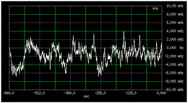
Fig 3.7.1.11 Frequency deviation, fast loop (qer_p=-19000 qer_d=-200000), 2mHz/div , antenna "A"
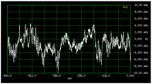
Fig 3.7.1.12 Frequency deviation, fast loop (qer_p=-19000 qer_d=-200000), 2mHz/div , antenna "B"
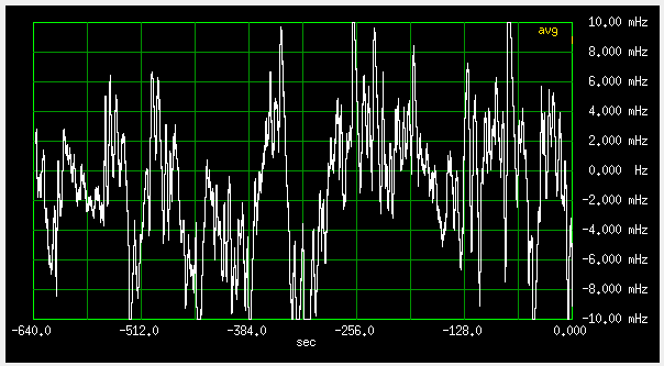
Fig 3.7.1.13 Frequency deviation, fast loop (qer_p=-19000 qer_d=-200000), 2mHz/div , antenna "C"
My assumption was, that the lower "B" antenna would see less ground (and no metal roof), so the wiggles would be smaller and slower. Maybe they are slower, but with the higher "C" antenna, they are even slower. So the ground reflection hypothesis seems less plausible now?
For more about multipath, see section four below.
What can be seen relatively well is, that the less sky the antenna sees, the worse is the short term stability. In fact, with "B" and "C", the deviations exceeded +-5E-10, and the clockd loop was kicking in, as can be seen on the error graphs:
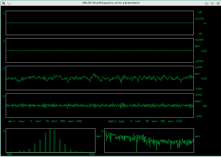
Fig 3.7.1.14 Error graphs, fast loop (qer_p=-19000 qer_d=-200000), 2mHz/div , antenna "A"
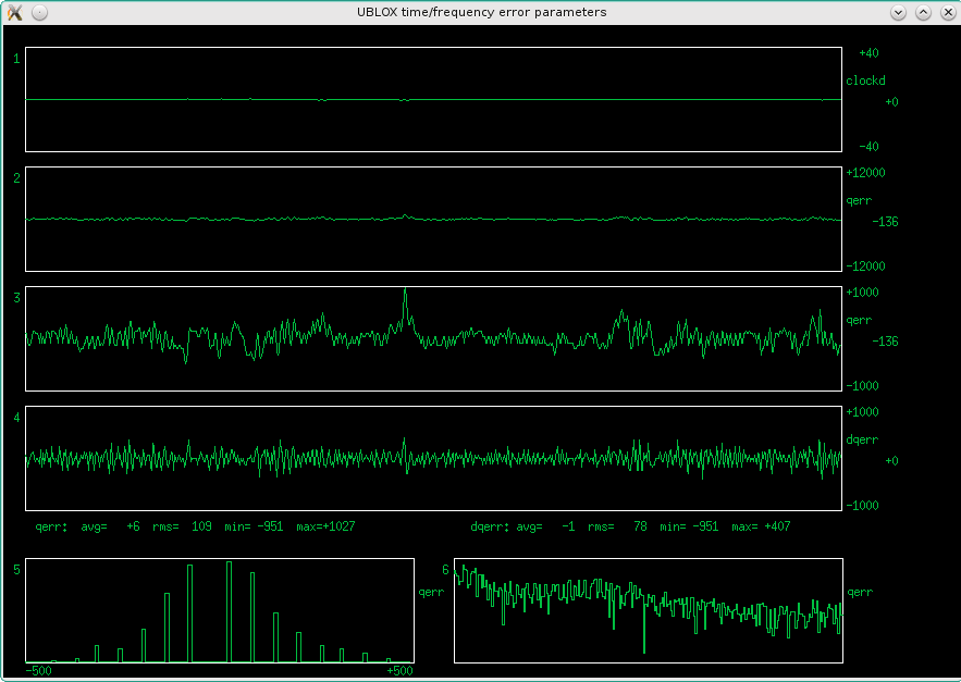
Fig 3.7.1.15 Error graphs, fast loop (qer_p=-19000 qer_d=-200000), 2mHz/div , antenna "B"
The missing "tooth" in the histogram is a "feature" of the ublox, happens rarely.
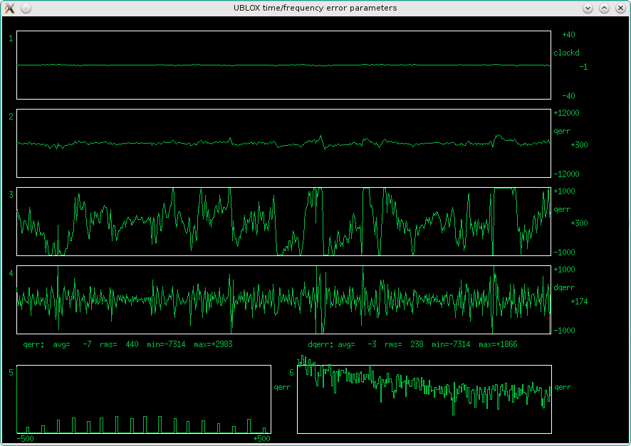
Fig 3.7.1.16 Error graphs, fast loop (qer_p=-19000 qer_d=-200000), 2mHz/div , antenna "C"
Up to table of contents
3.7.2 Signal levels
I did not do absolute level measurements, just checked whether I am enough over the threshold, and how weak GPS signal influences the short term stability.
To do that, I repeated the same tests as above, this time always with antenna "A", and inserted 6, 10 and 16dB of attenuation (taking care of DC, of course) at the receiver antenna terminal. These were the results:
Fig 3.7.2.1 Frequency deviation, fast loop (qer_p=-19000 qer_d=-200000), 2mHz/div , antenna "A", 0dB
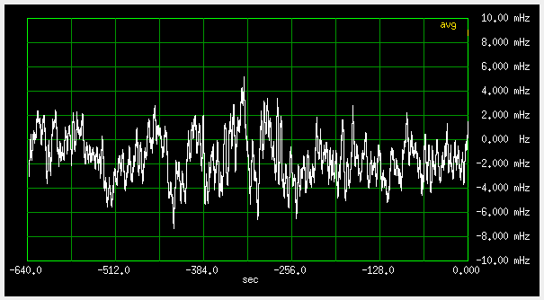
Fig 3.7.2.2 Frequency deviation, fast loop (qer_p=-19000 qer_d=-200000), 2mHz/div , antenna "A", 6dB
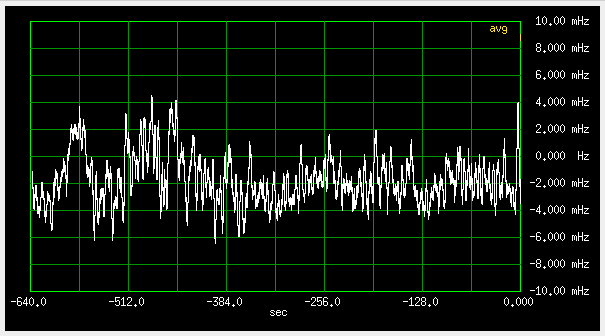
Fig 3.7.2.3 Frequency deviation, fast loop (qer_p=-19000 qer_d=-200000), 2mHz/div , antenna "A", 10dB
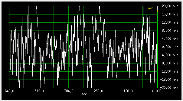
Fig 3.7.2.4 Frequency deviation, fast loop (qer_p=-19000 qer_d=-200000), 4mHz/div , antenna "A", 16dB
Inserting 6 and 10 dB makes little change, meaning that the active antenna has enough gain, to cover cable loss and receiver noise quite well. Only a slight increase in high frequency noise (the "line thickness") can be seen. The S/N is mostly determined at the first amplification stage in the antenna, as it should be.
The slower wobbles, at approx 100 second scale, do not seem to be influenced by the attenuation. A hint, that they are intrinsic to the GPS system, and not due to the receiver noise.
At 16dB attenuation, things start to fall apart. The loops keep tracking, but struggle. Still, the slower wobbles do not increase.
Up to table of contents
3.8 (Preliminary) conclusions
The MBSD comes quite close to the "as good as possible" solution, limited by the properties of the GPS signal itself, and the quality of the "flywheel" OCXO.
In the slow loop version, the frequency tends to stay within +-1E-11, but the timing is undefined.
The medium loop version sacrifices some short term frequency stability, to fix the time.
The fast loop version tracks the GPS signal tightly, significantly spoiling the short term stability of the OCXO. Nevertheless, it is probably suited for some applications, since the commercial telecoms GPSDOs seem to be tuned this way.
The MBSD as-is, needs some spit and polish, and some slight improvements (described below) could still be possible. Other than these, a better "flywheel" is more or less the only way to achieve significant improvements.
I do plan to try locking a rubidium, but the ones I have have worse phase noise than the HP OCXO, so I will probably try a "triple loop" (GPS, rubidium, OCXO).
3.9 Possible improvements
The MBSD, even in the current hacked-together form, measures up very well with other GPSDOs, but there is always room for improvement.
This is a list of things I haven't yet tried:
- 1. Use a real DAC instead of PWM
- 2. Use something less obsolete than ublox NEO-6M
- 3. Use a "T" type (timing) ublox receiver
- 4. Use a dual frequency receiver (ublox series 9...)
- 5. Adjust receiver parameters (min elevation, SBAS on/off...)
- 6. Better antenna (various groundplanes, QFH, etc.)
Before doing the above things, I wanted to have a solid working GPSDO, and see what and how I can measure, to estimate performance. That is also why I started with a simple KISS design, and only later moved to something more sophisticated.
Developing the MBSD, I certainly learned a pile of things, and developed some diagnostic tools. Next I want to design a PCB for the MBSD, and populate a couple of them, to have reliable hardware, no hanging wires. Need to think about what to put on the board, to make it versatile, before committing to FR4, so this will take some time.
When I'll have two MBSDOs, I will also try the "same antenna" measurements, like I did with the Trimble GPSDOs, as described on my
The ten mega party
page.
I already bought a couple of NEO-8T receivers on cut boards. Destroyed one while unsoldering (0201 components fell to the ground), the other (I hope) is still alive, haven't tried yet. These clock at 48MHz, so I will have to find a suitable 48MHz VCXO first.
The distributors offer many 48MHz "crystal oscillators", but most of these are in fact synthesizers in disguise. There are quite a few of these on offer, but most of them only in thousands quantities (whole reel). Mouser sells one in singles, but it is also a "non-stocked item".
Anyway, I want a "real" clean VCXO. So, I just ordered a bunch of 48MHz crystals from Ebay, and will try my hand at making a low noise VCXO.
Regarding antennas, currently I have no facility to measure antenna patterns, so I would be limited to just blindly try various antennas, don't like that.
On the firmware side, it would be nice to check the receiver status, satellite signal levels, jamming detection (an ublox feature), etc., and raise alarm if necessary.
Adding a second serial line for communication with a host computer would be desirable. MSP430G2553 only has one UART, but maybe a software UART could be added.
Some ublox modules also have a SPI port, which could potentially be used for communication with the MSP, to free the UART for host communication. On the Chinese boards I have, the SPI is not routed out.
Up to table of contents
4. Estimating time/frequency errors from position data
Having no absolute time/frequency etalon, what could be substituted?
I also do not know my "absolute" position, but at least I know my
antenna doesn't move anywhere, aside the plate tectonics :-)
Position errors can not be used to correct the timing output by the receiver, because
it is derived from multiple satellites at various directions in the sky. The receiver
could do it internally, because it has timing for each satellite separately.
Do Ublox T types do that?
Frequency deviations can be calculated from the time derivative of the position errors.
Analyzing a longer time record of measured positions, I can observe the deviations
from the average position, and from that, deduce what errors I should expect in the
time and frequency domains. Seeing the statistical properties of the errors, optimal
averaging could be proposed, for a given "flywheel" oscilator.
I did two longer records, one in June, when the Sun is high, one in September, around equinox,
and I will probably do one in December, when the Sun is low. They were done from antenna
"A" (see above).
The June recordings look like this:
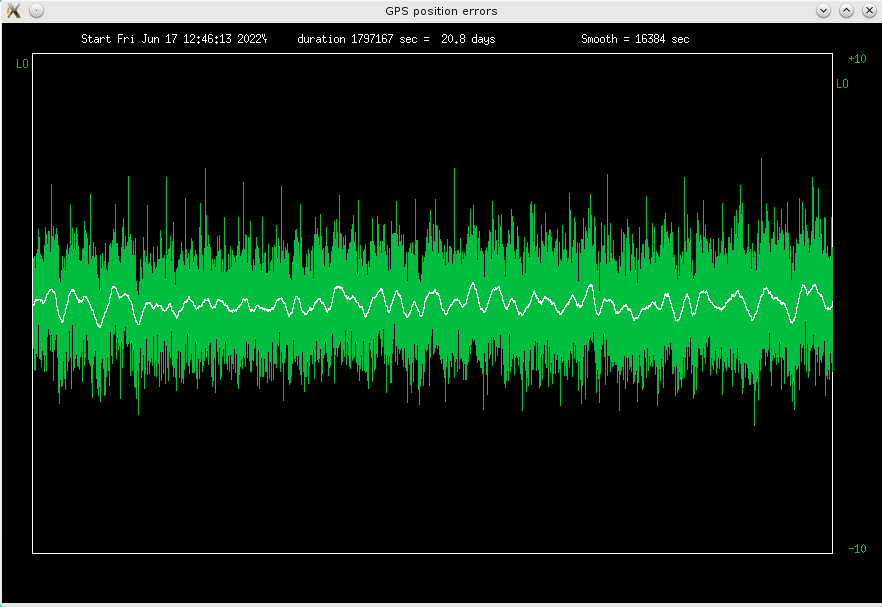
Fig 4.1 Deviations from average longitude, scale +-10m
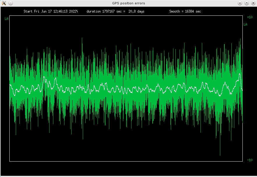
Fig 4.2 Deviations from average latitude, scale +-10m
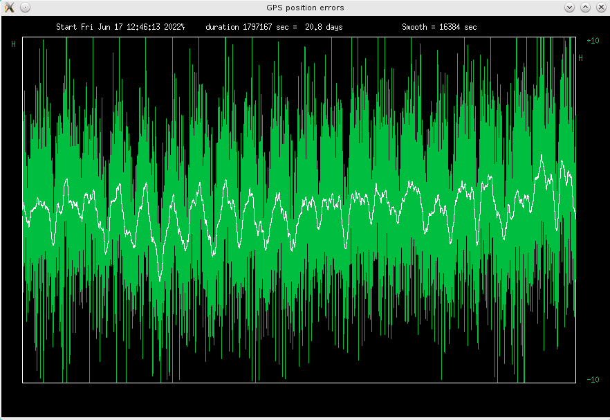
Fig 4.3 Deviations from average height, scale +-10m
The white curve is averaged over 16384 seconds (4.5 hours). The errors are the smallest
in longitude, and biggest in height. This is probably a matter of satellite geometry, at
46 degrees north.
RMS errors are 1.4m, 1.0m, 2.5m, peak errors +-8m, +-5.5m and +-12m for
latitude, longitude and height, respectively.
This are the September recordings:
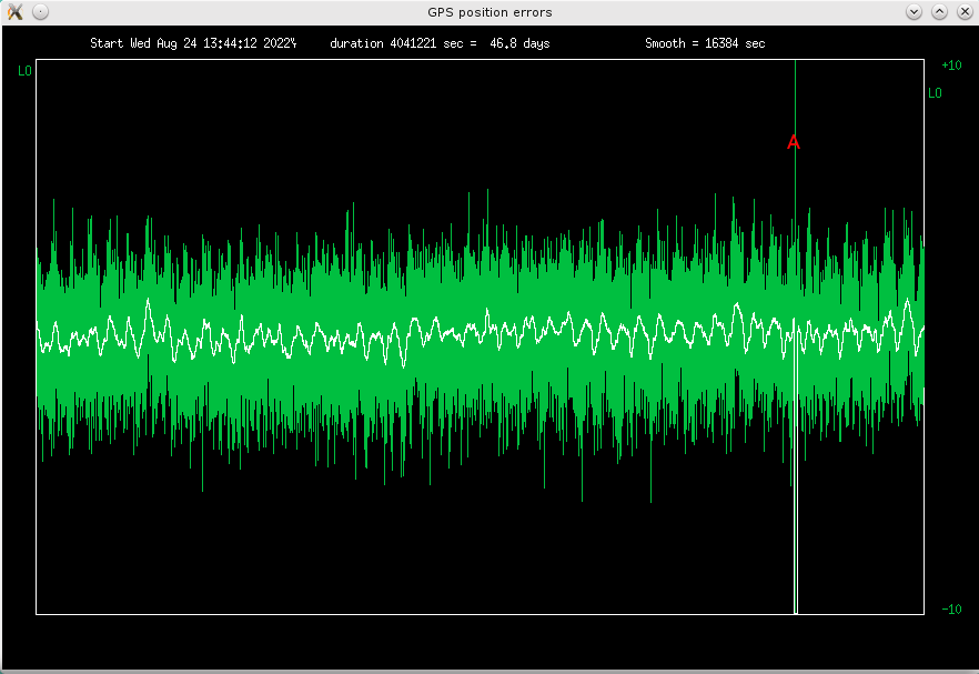
Fig 4.4 Deviations from average longitude, scale +-10m
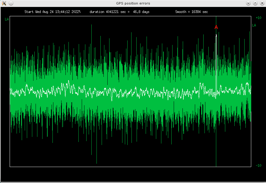
Fig 4.5 Deviations from average latitude, scale +-10m
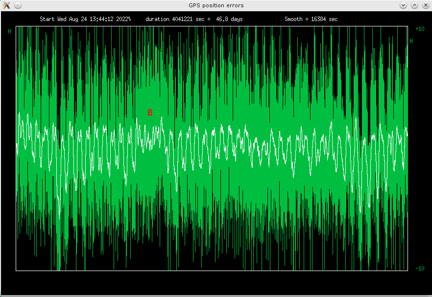
Fig 4.6 Deviations from average height, scale +-10m
There was a strange event (marked "A" in figs 4.4 and 4.5 above) on the third of October:
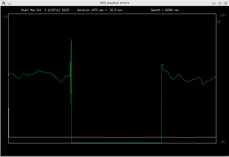
Fig 4.7 A glitch in the data (longitude shown, zoomed in)
Looks like you don't need to be in Ukraine to suffer GPS jamming - truckers use GPS
jammers to disable GPS trackers, installed on the truck by their bosses.
Since the outage lasted 15 minutes, it was not just a passing truck, but probably
a delivery truck, which stopped nearby.
Or what could it be?
The height seems unaffected in fig 4.6 above, but it was not:
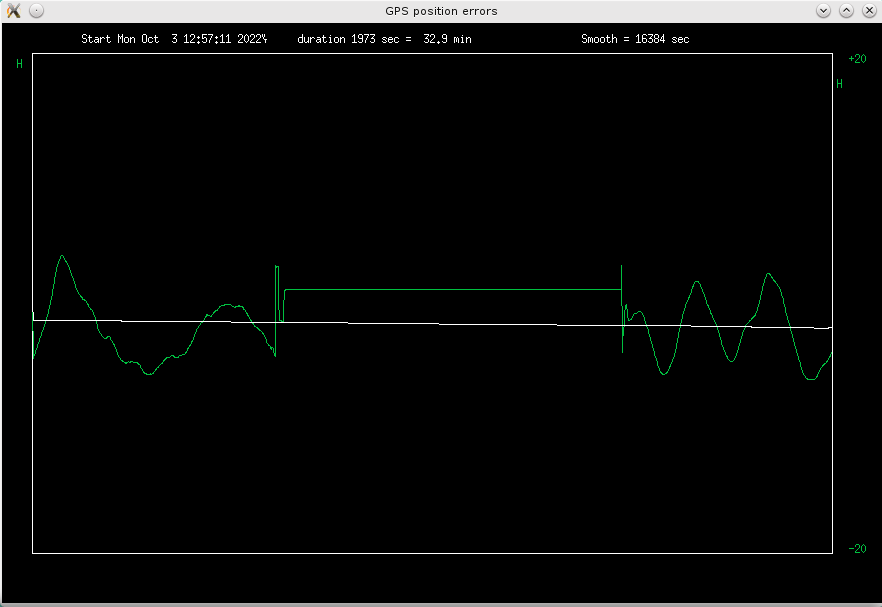
Fig 4.8 Jammed section of height data
Looks like the Ublox detects the jamming, and switches to the last good data point, and
holds it until it re-acquires the signal. Here, it was quite successful in height,
but not so much in latitude and longitude, where the errors are 157 and 365 meters.
Probably the oscillatory data at jamming start threw it off?
After removing the jammed section, the differences in the average position between June
and September were 20cm, 3cm and 156 cm in latitude, longitude and height.
Could the big difference in height be a seasonal thing? In June, the Sun is above horizon
much longer, so a larger amount of data is recorded during active ionosphere each day,
which might shift the average. I hope I can do the December recording!
The height seems to be the most affected by the ionosphere, as it has the biggest
24h periodic component (which sometimes misteriously disappears, B in fig 4.6).
Obviously, to do a site survey for a T-type Ublox, the averaging time should be a
multiple of 24h, to null out the daily variation.
Looking at fig 4.6 above, the tops of the curve (nights) seem to have less variation than the
bottoms (days), which is expected, since during the day, the ionosphere is exposed to
the variable Sun.
Could we profit from averaging only during nighttime? This would be doable with a
rubidium "flywheel" oscillator.
So I did 24h and night only
averages over the 45 days of the September recordings (height data is shown):

Fig 4.9 Green curve: 24h averages, yellow curve: night only averages (40000 seconds centered on midnight)
There is a difference, but not a big one: the RMS ripple reduces by about 18 percent,
to around half a meter, or 1.6 nanosecond. Peaks are about three times that, plus minus
1.5 meters or five nanoseconds. Per 24h, this would be about 6E-14 error in frequency.
Looking closer at the error graphs by zooming in time, many small wiggles with a period
of about a minute can be seen. This is about what one would expect from multipath,
which should repeat daily, when the satellites are in the same position. Drawing the
errors of two consecutive days, one can see some similarity, especially during night time:
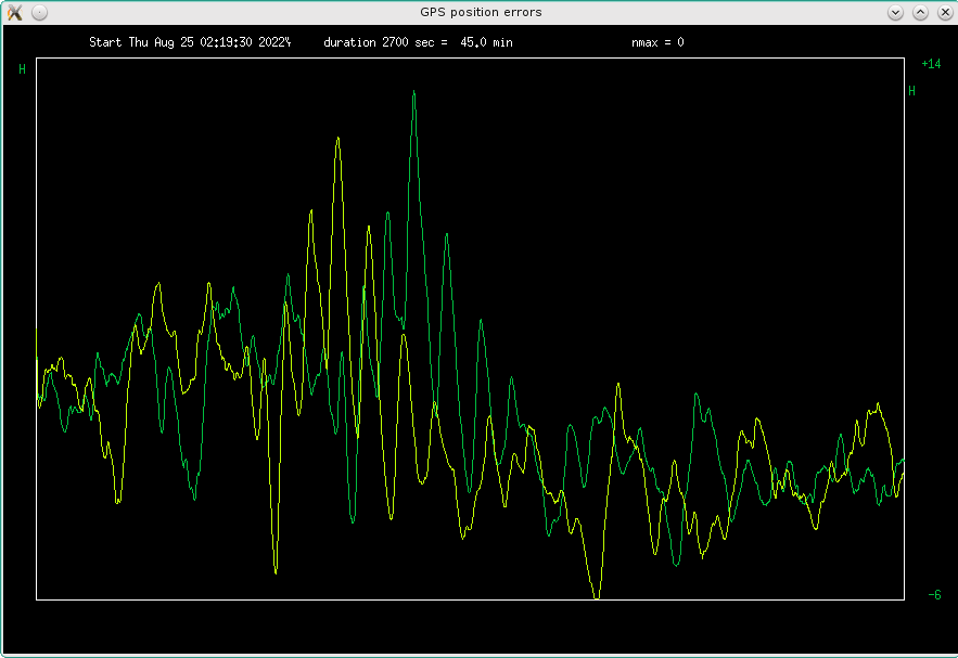
Fig 4.10 zoomed in time errors on two consecutive "Sun" days
with some offset. So I calculated the autocorrelation for 24h plus minus 500s offset:
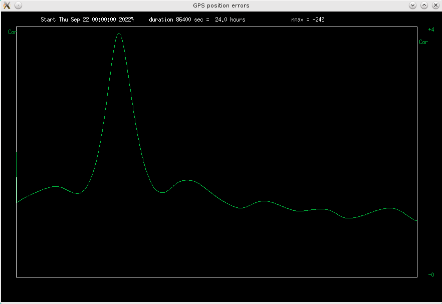
Fig 4.11 Autocorrelation of errors around 24h offset
There is a very nice hump at -245 seconds, which fits Earth rotation exactly. Plotting
now the two graphs with this offset, shows a remarkable similarity:
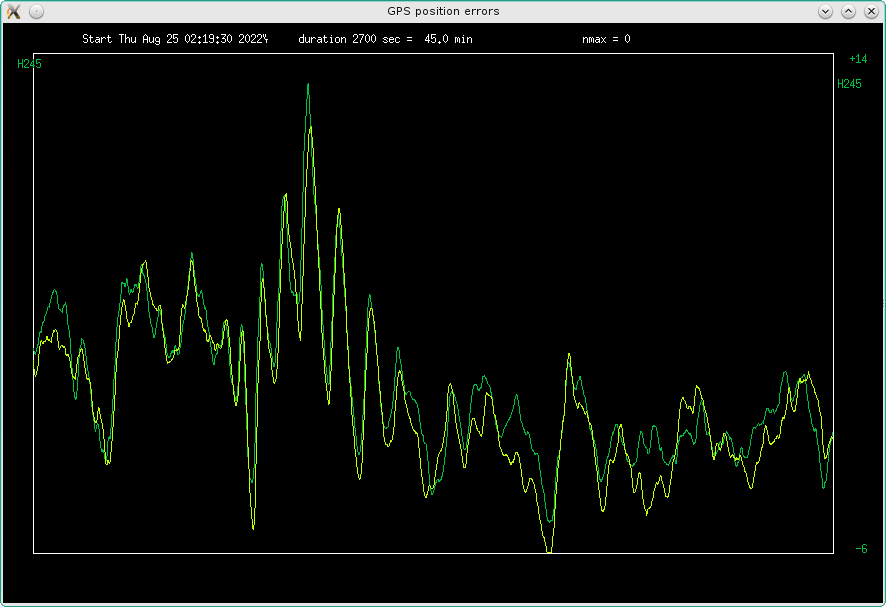
Fig 4.12 zoomed in time errors on two consecutive sideral days, nighttime
During the day, the ionosphere can shift things between two days (and there is a
parking lot with variable car distribution next door):
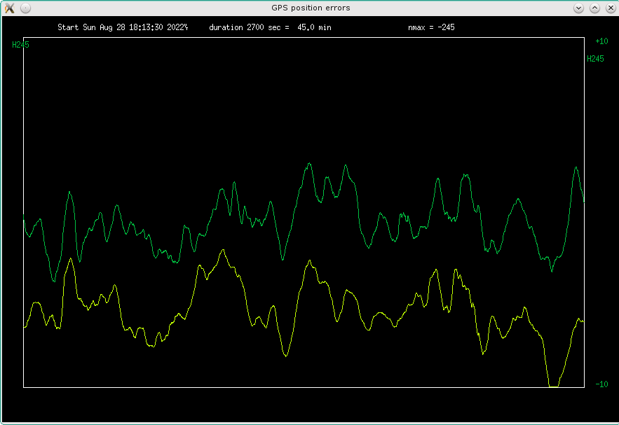
Fig 4.13 zoomed in time errors on two consecutive sideral days, daytime
but the ripples are still quite correlated.
Assuming the satellite orbits are quasi fixed in space, and the Earth rotates below them,
these wiggles are almost certainly multipath.
Would need to repeat this with the antenna on the ground, in the
middle of a meadow. But for that I would have to make a solar powered recorder, and find
a place, where I can leave it for a month, without it being stolen.
In fact the satellite orbits are about 12h, but you can't see that periodicity.
After 12h, the satellites will be in the same positions, but you won't. Well, except
if you are at the north or south pole, but you won't see many satellites there.
So, for an Earth bound observer, satellite positions repeat every two orbits.
The spectrum of the height errors:
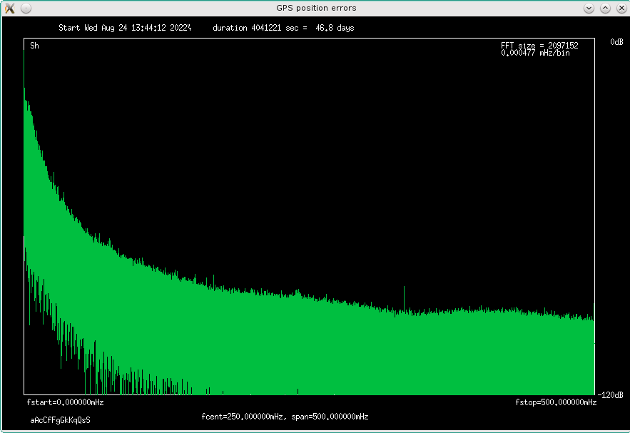
Fig 4.14 spectrum of height errors, September recording
is kind of 1/f-ish. Averaging mostly eliminates higher frequencies, so this is bad
news. The 1/24h component can not be seen, because the above graph is a million
FFT bins squeezed into 800 pixels, it is all crammed into the first pixel. Zooming
on to the lower frequencies shows it, with a comb of harmonics:
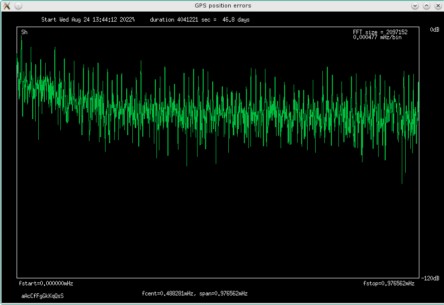
Fig 4.15 spectrum of height errors, zoomed in
In the end, I calculated a "Spatial Quasi Allan Deviation", by multiplying meters with
3.3 nanoseconds:
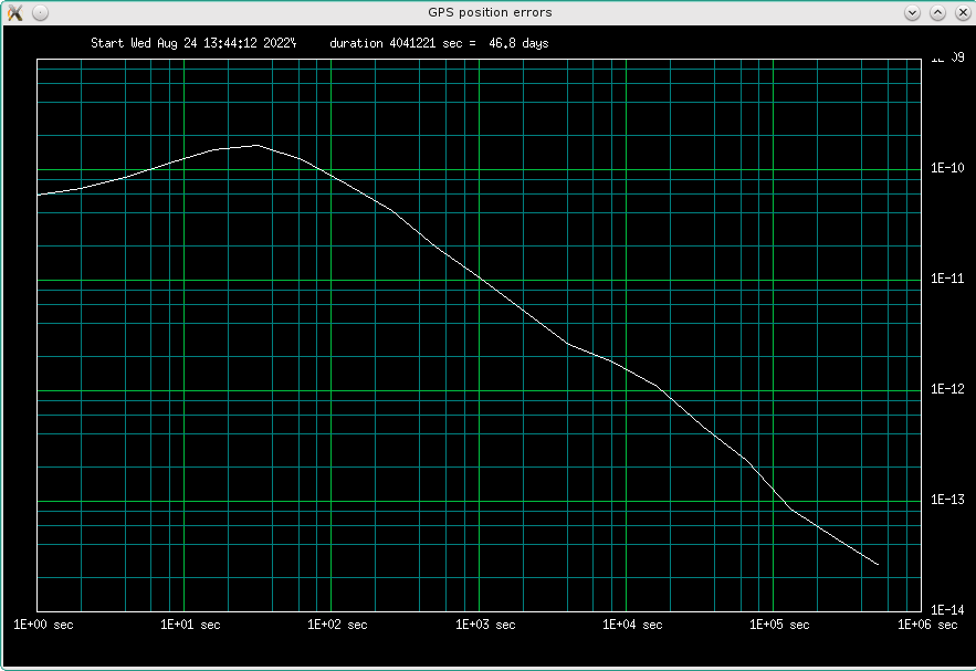
Fig 4.15 Spatial Quasi Allan Deviation, height data
I guess the peak around half minute is from those multipath wiggles.
In any case, it would be nice to repeat these measurements with different antennas,
and maybe with one of those dual frequency receivers (Ublox series 9...)!
Up to table of contents
5. Common antenna measurements
To estimate how much of the errors are contributed by the external factors, I connected two identical
GPSDOs to the same antenna (via a wilkinson power divider). Since I haven't yet made
more than one MBSD, I did this with the Trimble 65256 GPSDOs, of which I have two identical units.
Therefore, the results might not directly apply to the MBSD.
I found the Trimble GPSDO's outputs have a peculiar "jump once per second" form of noise.
Comparing the output with a free running HP10811 gives this:
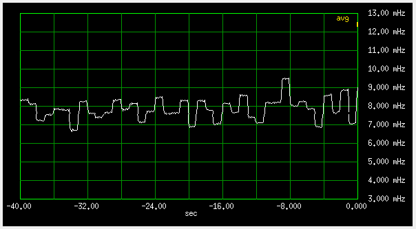
Fig 5.1
Next, I connected two of them to the same antenna. This should make all of the external
errors (ionosphere, multipath, interference, satellite errors...) the same for the two receivers.
I checked the signal level using attenuators, to ensure that the noise from the active
antenna dominated, so that more than 90% of the noise was also the same at receiver inputs.
Would they jump in unison now, drastically reducing the frequency difference between them?
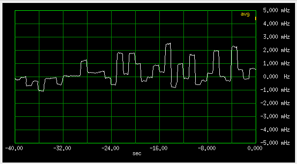
Fig 5.2 Frequency difference between two Trimble GPSDOs connected to the same antenna
Nah. Mierda!
So it seems, we are limited by internal noise. I should have expected that, since close multipath and the ionosphere do not change much on such short time scales.
However, the short time differences are still remarkable, considering that more than 90% of
receiver noise was also the same.
I guess one explanation is, that the two GPSDO's
have independent free-running clocks, so the sampling points of the input A/Ds do
not coincide (a MBSDO would be better in this respect?)
The rounding in the following low bit number integer signal processing then amplifies
that noise. I assume low bit number integer processing, because these chips implement hundreds of
correlators with very low current consumption.
The once per second jumps also make a hump at one second in the short times ADEV curve:
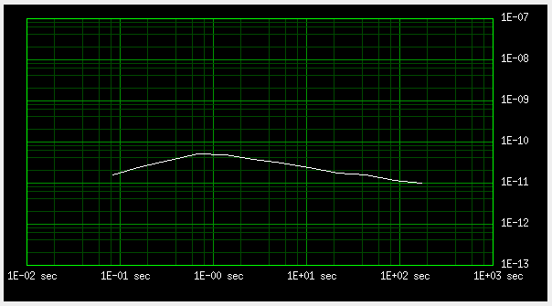
Fig 5.3 ADEV between two Trimble GPSDOs connected to the same antenna, short times
I only calculate ADEV once per octave (a little more than three points per decade), so the hump looks wide.
As expected, on larger time scales, the ADEV curve plunges down into oblivion, because, in the end, both 10 MHz outputs are derived from the same clock (the GPS signal on the common antenna).
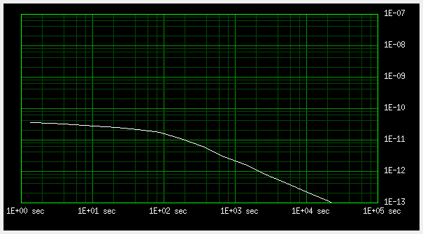
Fig 5.4 ADEV between two Trimble GPSDOs connected to the same antenna, longer times
The mutual phase flaps around by about plus minus 200 milliradians (+-12 degrees).
Is there some drift in the data? This would be a hint, that these GPSDOs are FLLs, not PPLs.
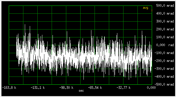
Fig 5.5 Plot of mutual phase over two days
Note that the four curves above show the sum of contributions from both GPSDOs. Assuming their contributions are equal, the amount from each one separately would be somewhere between 50 and 71% of the total, depending of the amount of correlation between the two. There will be correlation, because of the common noise from the active antenna and its surroundings is dominant.
Next, I tried frequency difference measurement on medium time scales, with common and separate antennas. (Antennas A and B, as described in the
antenna positions section above.)
During 21 minutes, it looks like this:
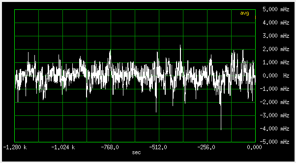
Fig 5.6 Frequency difference, common antenna
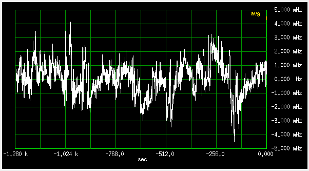
Fig 5.7 Frequency difference, separate antennas
The difference is bigger, because the noise is now uncorrelated, and maybe some multipath. The ionospheric effects shouldn't be significant at such small antenna spacing and time scale.
With separate antennas, the hill on the ADEV is higher, and shifted to longer times:
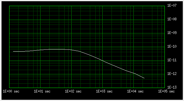
Fig 5.8 ADEV, separate antennas
6. Microcontroller programming
TI offers a big selection of MSP programming tools. I'm a cheapo guy, so
I am using an "launchpad" MSP-EXP430G2 emulation board. I think TI stopped producing this particular model, but they are still widely available at ebay etc, although prices are rising - originally it cost about ten euros. An almost identical substitute from TI is the MSP-EXP430G2ET, for ten bucks. Alternatively, TI is making other similar boards, which could probably be used. Look for one that does "SPI by wire" programming, because I do not bring out the full JTAG wire set.
MSP-EXP430G2 can be used to program the MSP430G2553 in two ways: either plug it into the onboard socket and program, or connect four wires, and do in-circuit programming.
NOTE: for socket programming, the jumpers must be on. For in-circuit, the socket must
be empty, or else remove the jumpers.
With other "launchpad" boards, only in-circuit programming will be available, because on them the SMD MCU is soldered, no socket.
For "SPI by wire" in-circuit programming, the following four wires are needed:
- 1. Vcc 3.3V
- 2. RST (reset)
- 3. TEST
- 4. Ground
On my boards with MSP microcontrollers, I provide a 4 pin connector, with pin numbers as above, labeled "+RTG". Pin 1 is the square pad (see J2 in fig. 32 above).
For programming, I use the
mspdebug (external link) software under Linux. The exact command is in the comments at the beginning of each program file. The compilation command for the msp430-gcc compiler is also given there.
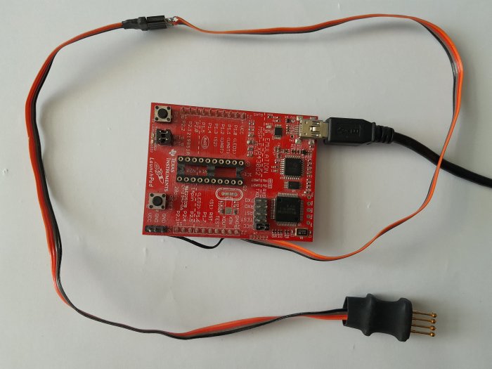
Fig 71. MSP-EXP430G2 with 'SPI by wire' wires and pogo pin extension
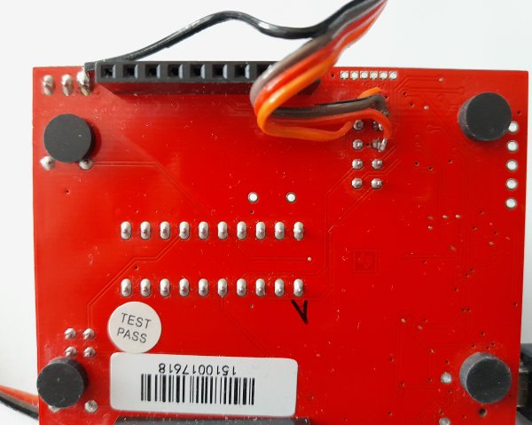
Fig 72. 'SPI by wire' wire connections
Up to table of contents
7. Downloads
I want to make this a fully open design, schematics, PCBs, firmware et all. If you find something missing, ping me.
7.1 KISS versions
I do not recommend you to build these, I did not design a PCB for them, etc. But if you want to experiment, here is the stuff:
Kicad project (schematic only)
KISS v1 firmware v0.1
KISS v2 firmware v0.1
7.2 The MBSDO
PLL frequency converter (VCXO synth):
Kicad project
Firmware v0.1
MBSDO:
Kicad project (not yet finished)
Firmware v0.1
Up to table of contents
8 References and literature
[1] MIS24N's GPSDO design on EEVblog:
http://www.eevblog.com/forum/projects/budget-gpsdo-a-work-in-progress/msg3481886/#msg3481886
[2] Lars' GPSDO design on EEVblog:
https://www.eevblog.com/forum/projects/lars-diy-gpsdo-with-arduino-and-1ns-resolution-tic/
[3] Simon Schroedle's GPSDO design:
http://www.simonsdialogs.com/2018/10/u-blox-gps-receiver-a-self-regulating-clock-and-a-gpsdo-and-all-of-this-for-the-lowest-cost
[4] u-blox LEA8F:
http://www.u-blox.com/en/product/lea-m8f-module
[5] N8UR evaluation of LEA8F:
https://hamsci.org/sites/default/files/publications/2020_TAPR_DCC/N8UR_GPS_Evaluation_August2020.pdf#page=17
u-blox timing application note:
https://www.u-blox.com/sites/default/files/products/documents/Timing_AppNote_%28GPS.G6-X-11007%29.pdf
u-blox 6 interfacing:
https://www.u-blox.com/sites/default/files/products/documents/LEA-NEO-MAX-6_HIM_%28UBX-14054794%29_1.pdf
u-blox 6 receiver and protocol description::
https://www.u-blox.com/sites/default/files/products/documents/u-blox6-GPS-GLONASS-QZSS-V14_ReceiverDescrProtSpec_%28GPS.G6-SW-12013%29_Public.pdf
https://www.u-blox.com/sites/default/files/products/documents/u-blox6_ReceiverDescrProtSpec_%28GPS.G6-SW-10018%29_Public.pdf
EEVblog, other discussions about GPSDOs:
https://www.eevblog.com/forum/projects/ebay-u-blox-lea-6t-gps-module-teardown-and-initial-test/
https://www.eevblog.com/forum/projects/my-u-blox-lea-6t-based-gpsdo-%28very-scruffy-initial-breadboard-stage%29/
https://www.eevblog.com/forum/projects/ublox-lea-m8t-module-to-discipline-an-external-oscillator/msg4471393/#msg4471393
https://www.eevblog.com/forum/projects/gpsdognssdo-stm32g4-u-blox-zed-f9t-tdc7200/msg4341235/#msg4341235
Up to table of contents
Up to S57UUU Home Page