Practical cavity filters for the frequency range 1GHz...4GHz
Matjaž Vidmar, S53MV
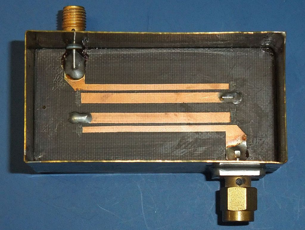
Band-pass electrical filters have different requirements for the manufacturing technology and dimensions of the final circuit. The filter bandwidth and its insertion loss together require a certain unloaded Q of the resonators to be used in the band-pass filter. The unloaded Q of lumped elements, especially coils, usually limit the unloaded resonator Q to below 100. The unloaded Q of microstrip resonators is not much higher due to both conductor and dielectric losses of the printed-circuit board in the frequency range around 1GHz:
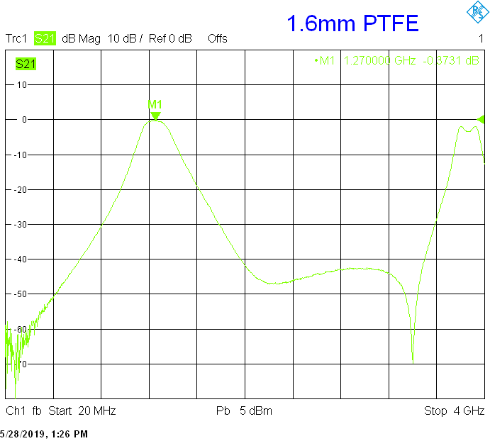
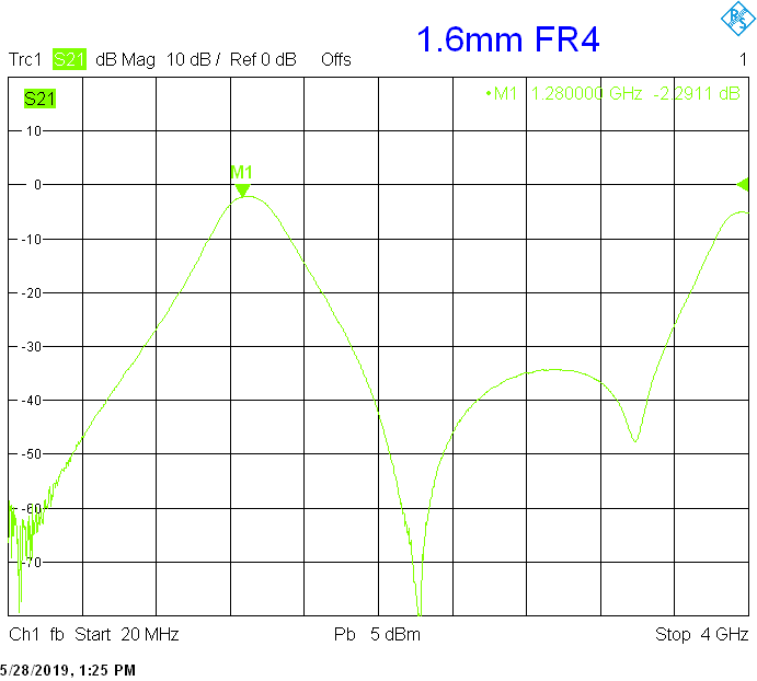
For example, the above-shown microstrip filter with two quarter-wavelength resonators built on 1.6mm thick teflon laminate can only achieve a bandwidth of 200MHz at a 1.27GHz with an insertion loss of about 0.4dB. If the same filter is redesigned to 1.6mm thick FR4, the insertion loss degrades to about 2dB. Finally, if the same filter is further redesigned to 0.8mm thick FR4, the insertion loss further degrades above 3dB!
Electrical cavity resonators are larger and heavier but can achieve a much higher unloaded Q. The unloaded Q of quarter-wavelength coaxial cavities may exceed 1000. The Q of larger microwave cavities may exceed 10000. The Q of optical cavities may exceed 1E+8. Electrical cavity resonators are usually much larger than their lumped or microstrip counterparts. The manufacturing of electrical cavity resonators may require a considerable amount of work and specialized tools.
Dielectric losses are almost inexsistent in hollow cavities. Conductor losses are the lowest for round or cylindrical conductor shapes. On the other hand, conductor losses are the worst in thin metal strips including microstrip circuits on printed-circuit boards. A good compromise that is also easy to manufacture are cylindrical wires inside a rectangular box.
All resonators have many additional resonant modes besides the desired resonant mode. In the case of electrical cavity resonators the frequencies of some undesired responses may be very close to the frequency of the desired response of the filter. Undesired responses have to be considered in all filter designs.
In the frequency range between 1GHz and 4GHz, quarter-wavelength cavity resonators have reasonable dimensions yet providing at least an order of magnitude higher unloaded Q than lumped components or microstrip circuits. A practical solution is to install a metal finger inside a hollow metal box or tube. Both the finger and the box or tube must be made from good electrical conductors like copper or aluminum. A quarter-wavelength resonator has one end of the finger connected to the box wall or tube wall while the other end is left open. Such a structure is self supporting and very rugged.
A band-pass filter usually requires many resonators. The coupling among different resonators has to be carefully adjusted for the desired filter response. In the case of quarter-wavelength resonators many metal fingers can be arranged inside a single metal box. Considering the coupling between adjacent resonators there are two basic band-pass filter designs: interdigital and comb:

Both interdigital and comb designs have a similar electrical equivalent circuit. Both interdigital and comb designs use electric (C') and magnetic (M) couplings between adjacent fingers. Both electric (C') and magnetic (M) couplings are of a similar magnitude. The effects of electric and magnetic coupling may add or subtract.
There is a subtle but very important difference between interdigital and comb filter designs. The phase of the magnetic coupling (M) alternates in an interdigital design, note the alternating red dots on the drawing. The phase of the magnetic coupling (M) stays the same in a comb design, all red dots are on the same side.
Since the electric coupling (C') leads 90 electrical degrees while the magnetic coupling (M) lags 90 electrical degrees, the effects of electric (C') and magnetic (M) couplings sum in an interdigital design. On the other hand, the effects of electric (C') and magnetic (M) couplings subtract in a comb design. If the same spacing between adjacent fingers is used, the interdigital design gives a stronger coupling and a wider filter pass-band. On the other hand, the comb design gives a weaker coupling and a narrower filter pass-band.
With ideal quarter-wavelength fingers the electric (C') and magnetic (M) couplings between adjacent fingers might cancel completely in a comb design resulting in zero coupling. In practice open-end effects (open-end capacitances) both require shorter fingers than lambda/4 and provide non-zero coupling in an comb design. Additional coupling is achieved in microstrip (air+dielectric) comb designs due to differing odd/even mode velocities.
In practice a comb design yields a more compact (smaller) filter than an interdigital design for the same center frequency, bandwidth and insertion loss. On the other hand, interdigital designs are simpler to scale to a different center frequency and/or different available hardware like finger (rod) diameter and/or box (tube) size.
In this article several practical filter designs are presented for the frequency range between 1GHz and 4GHz. All filters have three resonators. The coupling between adjacent resonators is a comb design. The input and output require stronger coupling, therefore the probes are coupled in an interdigital arrangement to the resonators:

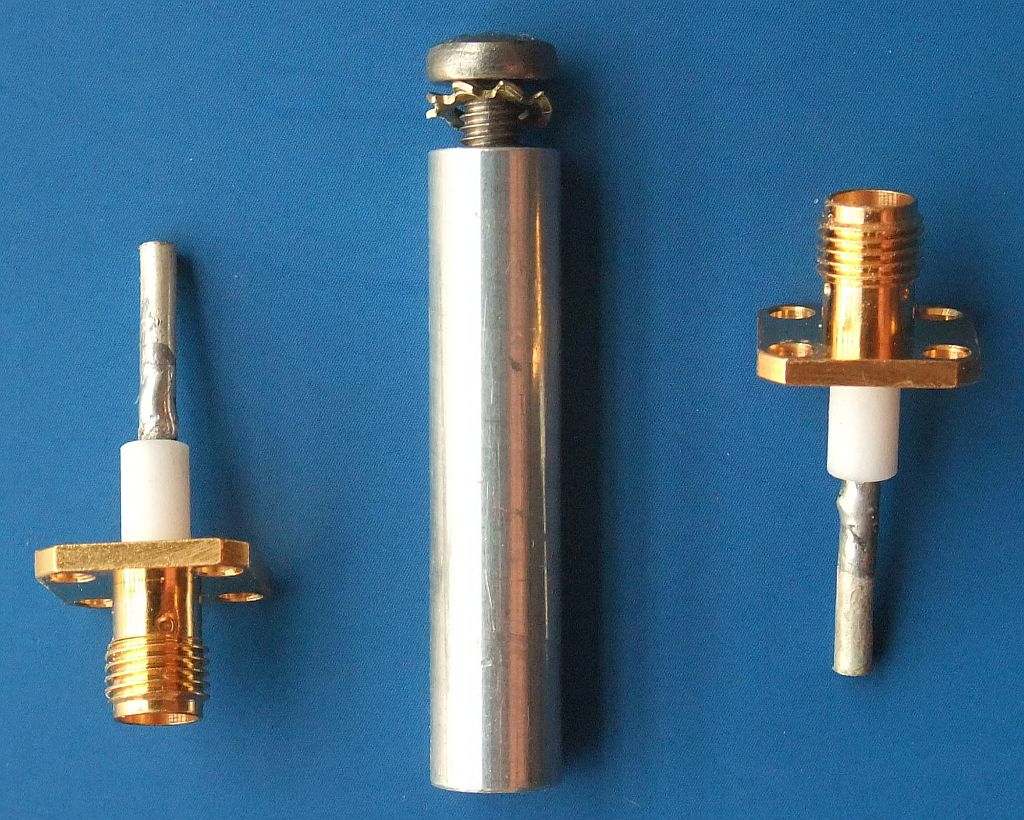
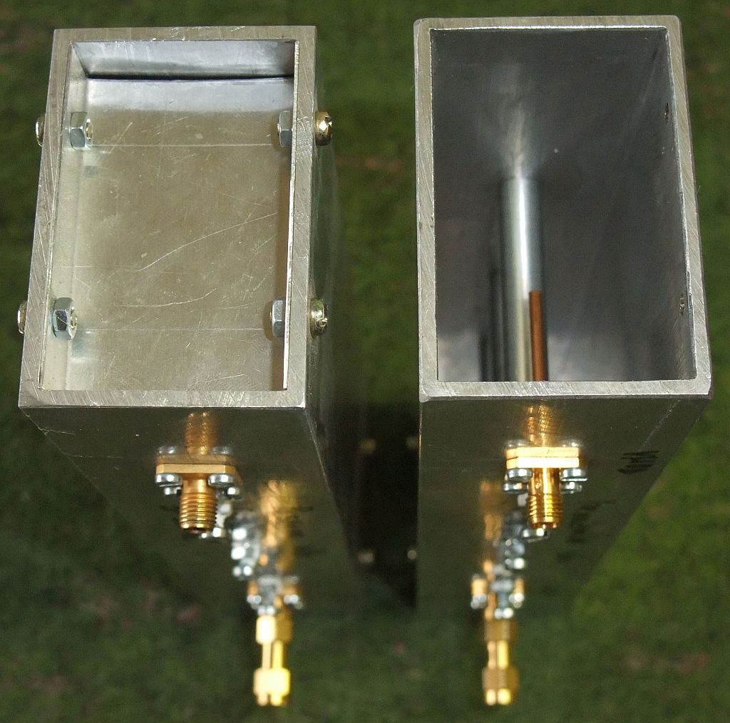
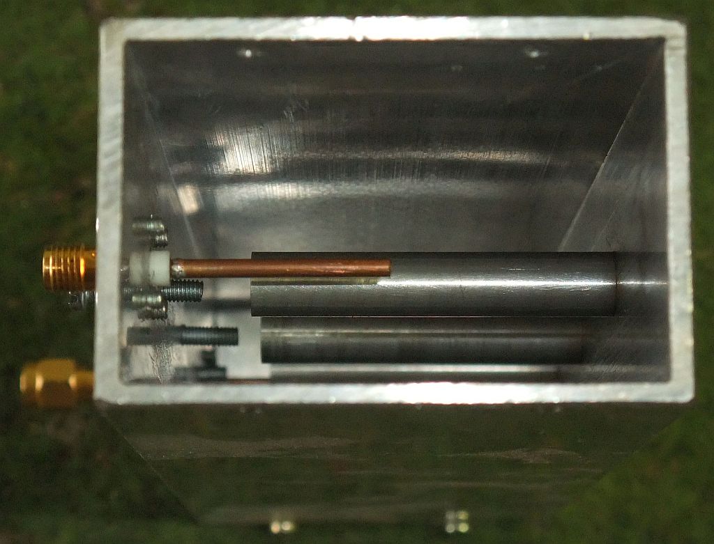
The fingers and probes are arranged inside an aluminum tube of rectangular cross-section. The tube cross-section is chosen to avoid rectangular-waveguide modes in the frequency range of interest. The fingers are made from aluminum rod and are attached to the tube wall using M4X10 screws. The coupling probes are made from thin copper tube (around 2mm diameter, in practice UT-085 semirigid shield) soldered to the center pin of a female SMA connector. The SMA connectors have rectangular flanges with four 2.6mm-diameter holes arranged in a 0.34"X0.34" square (8.6mmX8.6mm), installed on the tube wall with four M2.5X5 screws each:
In order to achieve a high unloaded Q of the resonators and stable filter performance it is necessary that all aluminum parts are in a good electric contact. In the proposed design it is sufficient to ensure a good electrical contact of the finger end to the tube wall. The latter should be aluminum to aluminum with no washers of any kind in between! Lock washers may be only be used outside the cavity under the screw heads to keep the latter from unscrewing.
The described quarter-wavelength resonator achieve their highest unloaded Q when the finger diameter (D) is about one third of the inner tube width (W'). In practice this can not always be achieved due to the available aluminum rod and tube sizes. Nevertheless the achievable Q has a broad peak as a function of the diameter-to-width ratio (D/W').
The rectangular aluminum tube has two open ends. If the tube ends are kept far enough (E) from the coupling probes, the evanescent electro-magnetic field decays enough that no covers are required. In practice it makes sense to make two covers from 0.6mm thick aluminum sheet to keep dust and dirt out of the filter cavity. Both covers are installed inside the tube and attached to the wide tube walls using four M3X6 screws each:
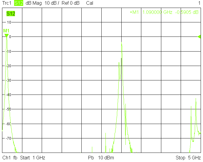
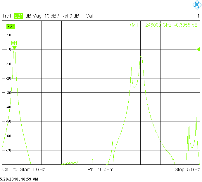
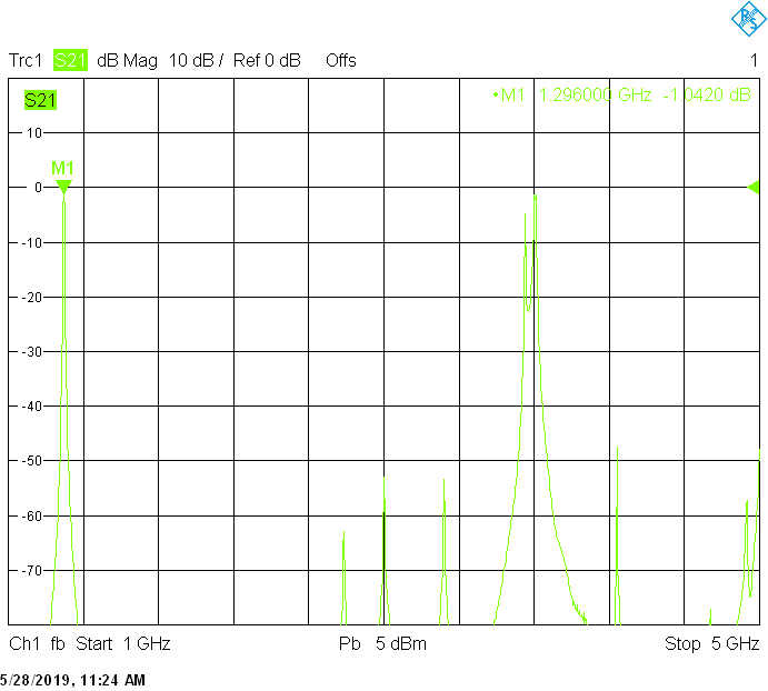
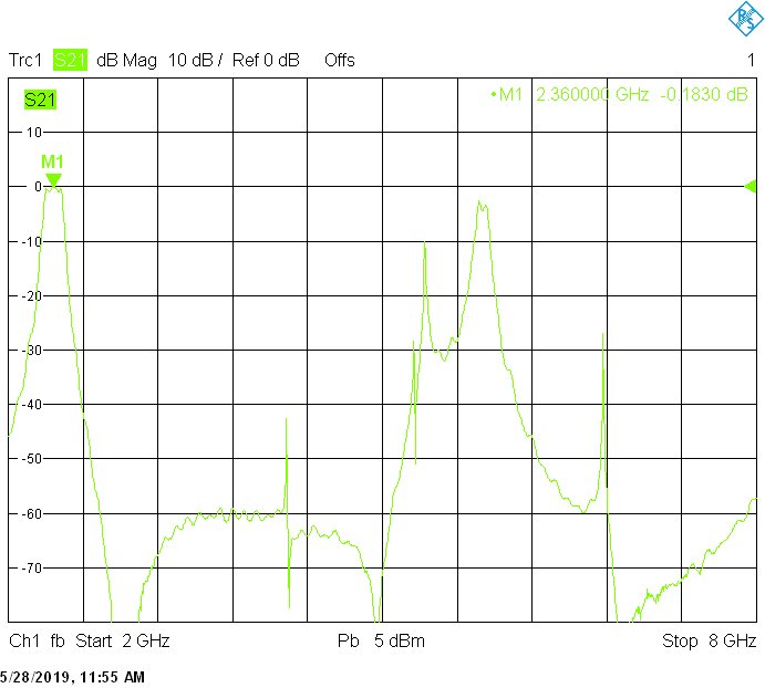
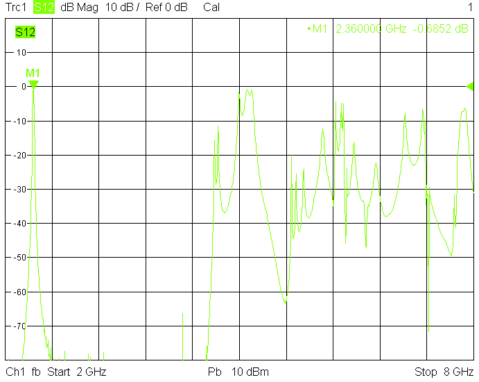
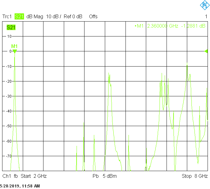
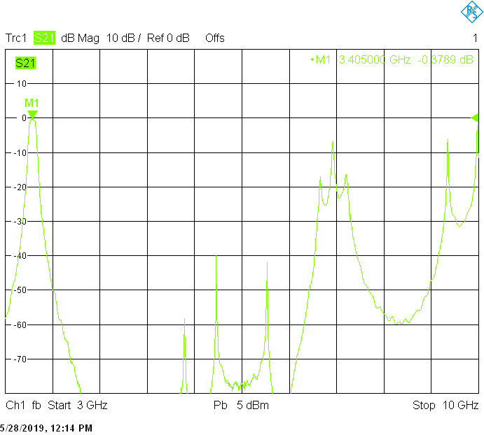
The unwanted responses of the described filters are caused both by waveguide modes inside the rectangular aluminum tube and by higher resonances of the fingers, in particular their three-quarter-wavelength resonance. The lowest unwanted response can be expected above f1=c/2H' (where c=3E+8m/s is the speed of light in air), but the latter is weak since it is only excited due to the constructional tolerances of the coupling probes. Of course these tolerances may change widely from one filter sample to another. Higher modes above f2=c/2W' and three-quarter-wavelength modes always provide strong unwanted responses.
The design parameters of several practically built and tested filters is shown in the following table:

The exact response of each filter is also a function of its tuning. The tuning is performed by small variable capacitors made from M3X15 tuning screws. The latter are screwed into threaded holes in the aluminum tubes to decrease the resonant frequency of each finger by approximately 5%. The useful tuning range of the complete filter is approximately +/-3% around its nominal center frequency. Of course filters can be tuned further down, but with the tuning screws very close to the finger ends the tuning becomes critical and the insertion loss increases. The tuning screws are held in position with a M3 counternut and lockwasher, both installed outside the filter cavity. On the finished filters it makes sense to lock the tuning screws in position with some paint:
The filter bandwidth is selected with the finger spacing (S). The latter is also a function of the inner tube dimensions (H') and (W'). The filter response can be optimized with the input and output coupling. Too weak coupling (probes too short) gives a three-peak response and increased insertion loss. Too strong coupling (probes too long) gives a single wide peak and increased insertion loss. Optimum coupling gives a nice flat-top response and minimum insertion loss:

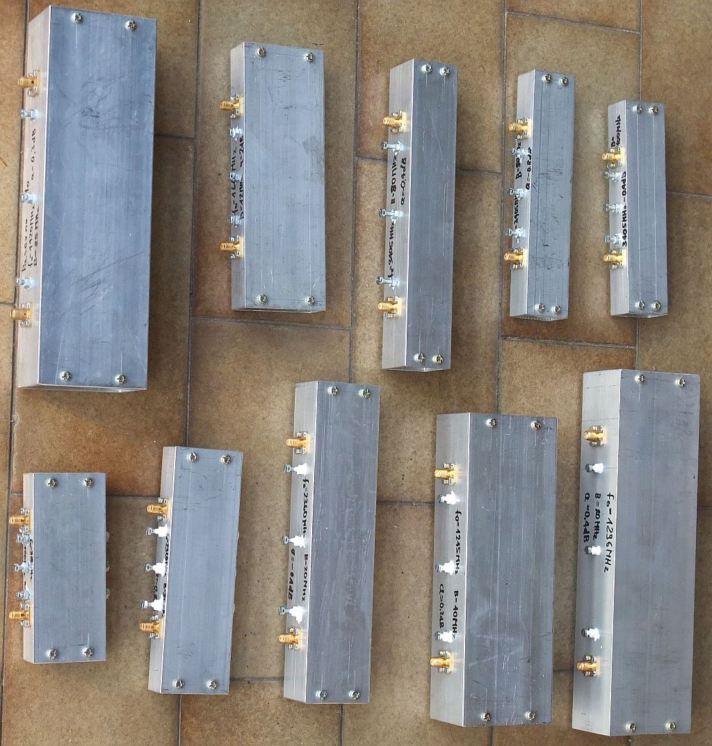
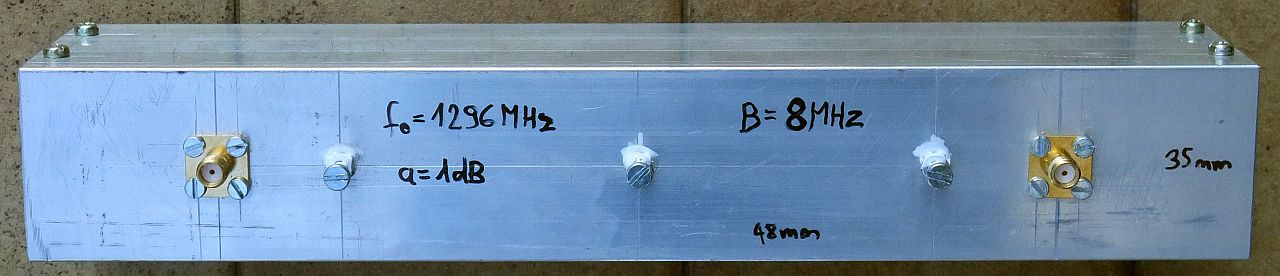
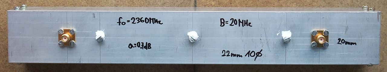
Several built and tested filters are shown on the following photo:
A filter for the 1.09GHz ADSB frequency band is built in rectangular aluminum tube with outside dimensions 60mmX40mm with 2.5mm wall thickness. Since this tube size is already tight for 1090MHz, shorter M3X10 screws are used for tuning:
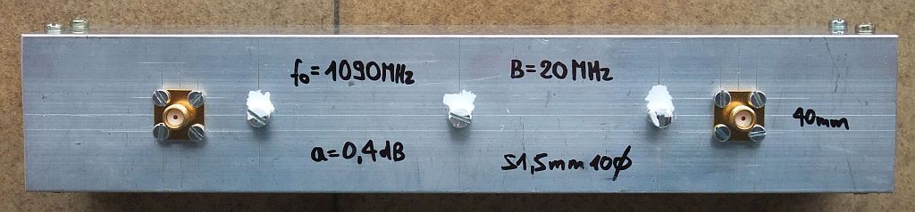
A 20MHz bandwidth is obtained with 50mm resonator spacing. The finite resonator Q already introduces a small insertion loss:
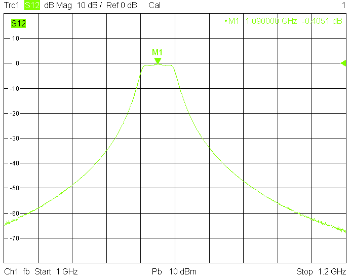
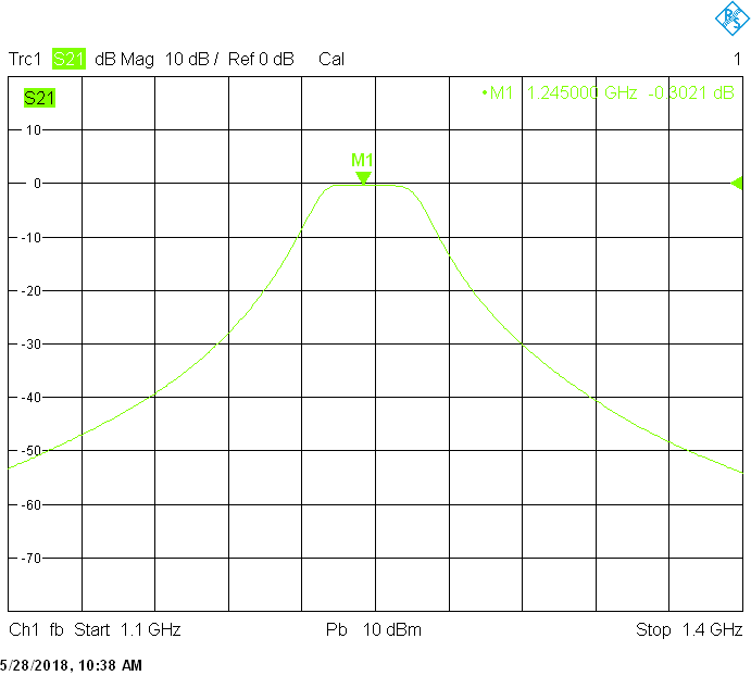
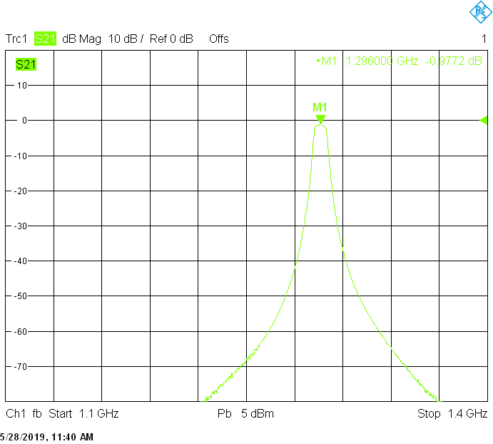
Filters for the 1.27GHz frequency band are built in rectangular aluminum tube with outside dimensions 60mmX40mm with 2.5mm wall thickness:
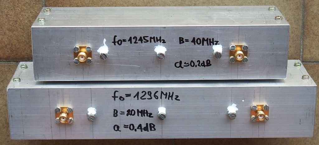
The 40MHz bandwidth version uses 40mm resonator spacing. Its insertion loss is very low and is mainly due to impedance mismatch:
The 20MHz bandwidth version uses 50mm resonator spacing. The finite resonator Q already introduces a small insertion loss:
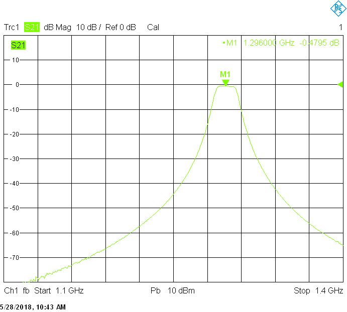
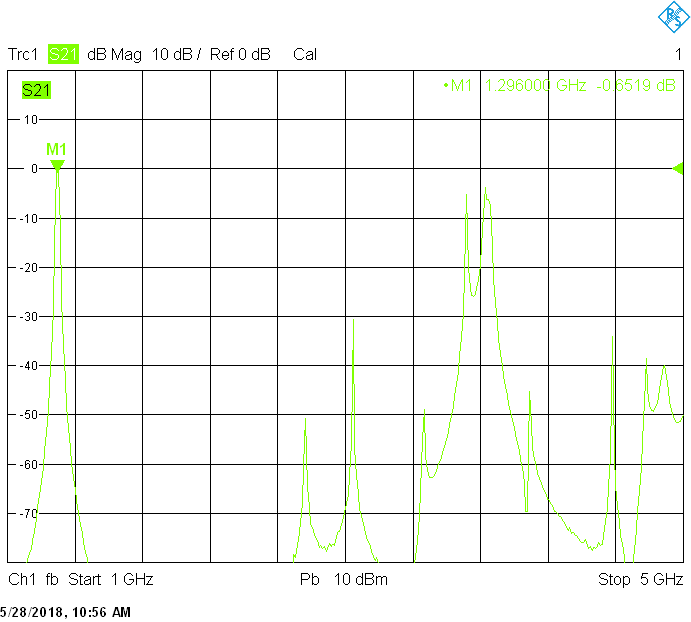
The 8MHz bandwidth version uses 60mm resonator spacing. The finite resonator Q already introduces a significant insertion loss:
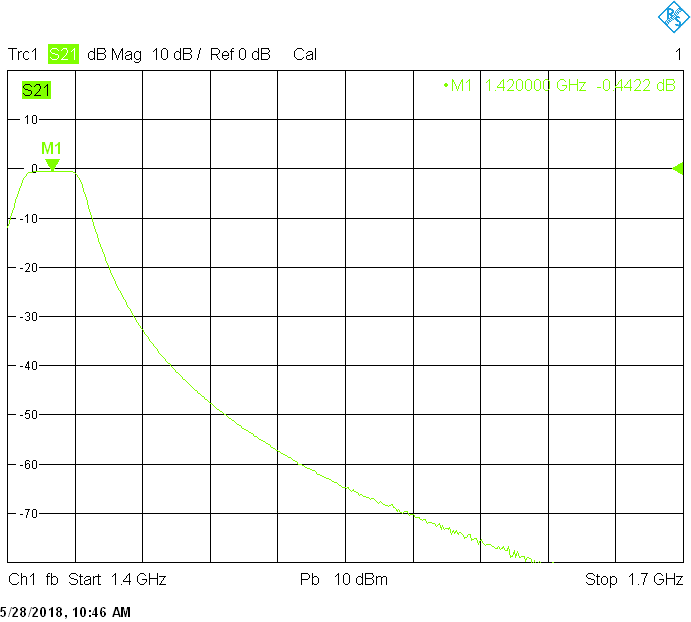
Filters for the astronomy frequency bands are built in rectangular aluminum tubes with outside dimensions 60mmX40mm with 2.5mm wall thickness and 50mmX20mm with 2mm wall thickness:
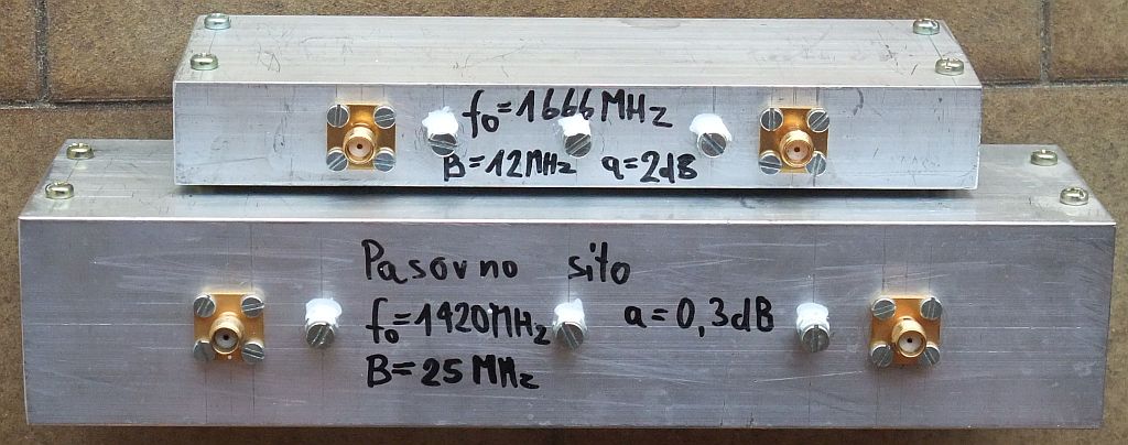
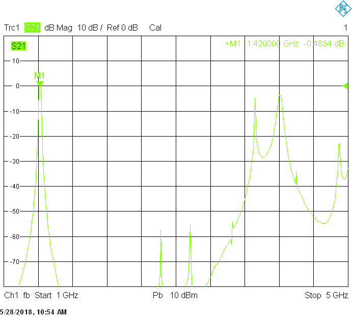
The 1420MHz version uses 45mm resonator spacing in a rectangular 60mmX40mm tube. The finite resonator Q already introduces a small insertion loss:
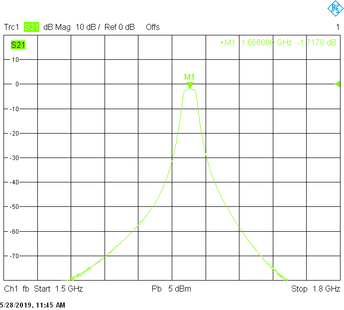
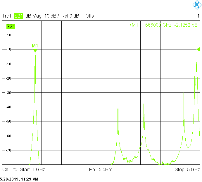
The 1666MHz version uses 25mm resonator spacing in a rectangular 50mmX20mm tube. The finite resonator Q already introduces a considerable insertion loss:
Filters for the satellite frequency bands are built in rectangular aluminum tubes with outside dimensions 50mmX30mm with 2mm wall thickness:
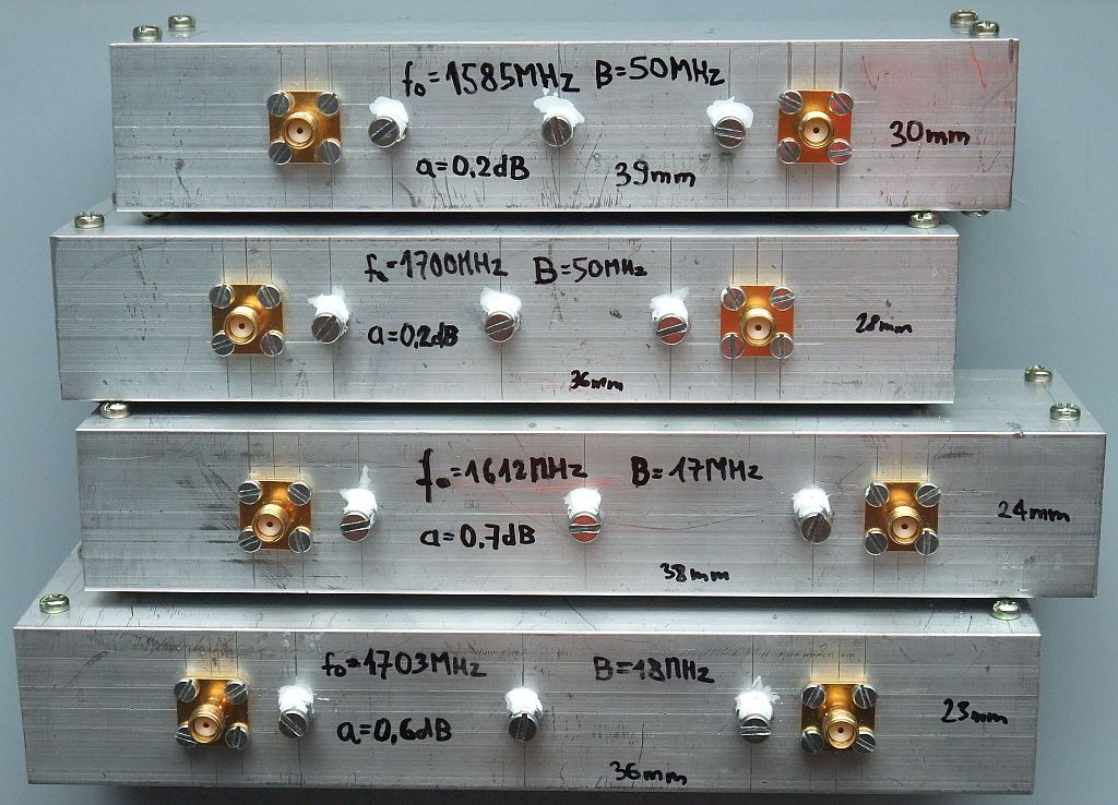
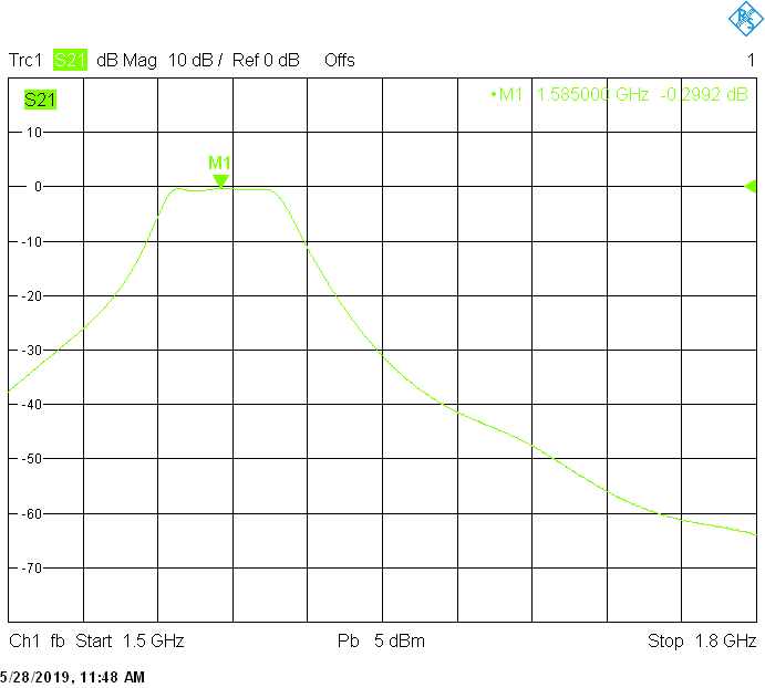
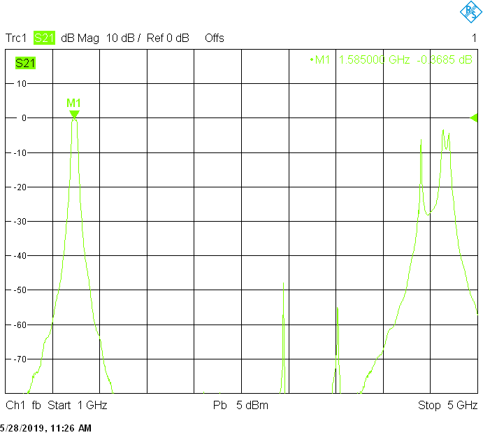
The 50MHz bandwidth version for 1585MHz uses 30mm resonator spacing. Its insertion loss is very low and is mainly due to impedance mismatch:
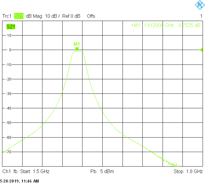
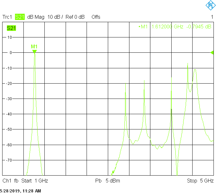
The 17MHz bandwidth version for 1612MHz uses 40mm resonator spacing. The finite resonator Q already introduces a small insertion loss:
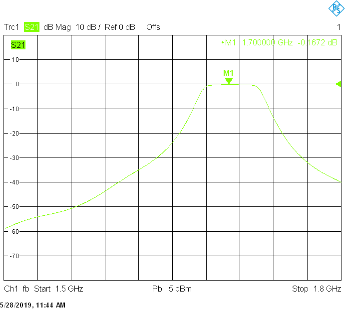
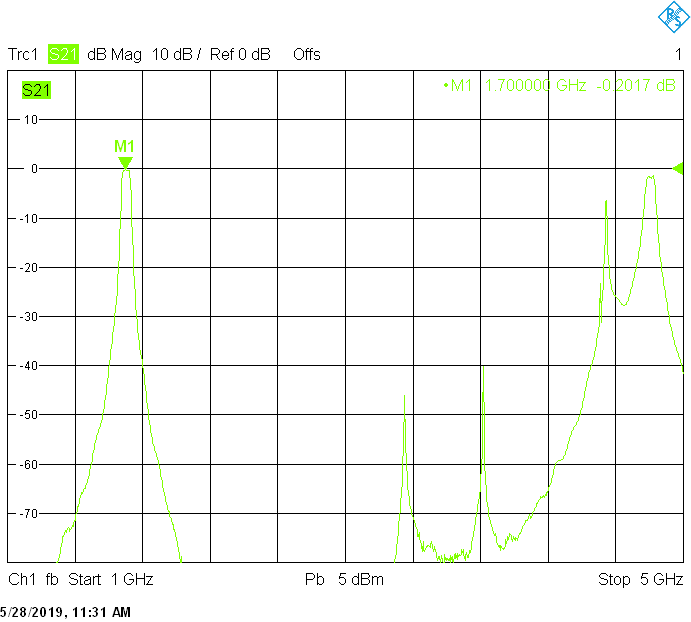
The 50MHz bandwidth version for 1700MHz uses 30mm resonator spacing. Its insertion loss is very low and is mainly due to impedance mismatch:
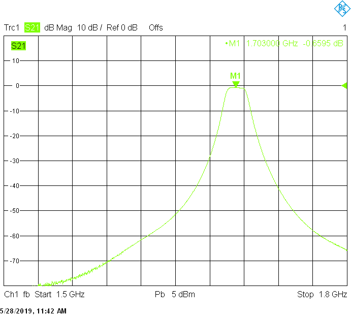
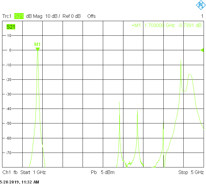
The 18MHz bandwidth version for 1703MHz uses 40mm resonator spacing. The finite resonator Q already introduces a small insertion loss:
Filters for the 2.3GHz frequency band are built in rectangular aluminum tubes with outside dimensions 40mmX20mm and 40mmX30mm both with 2mm wall thickness:
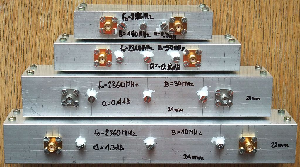
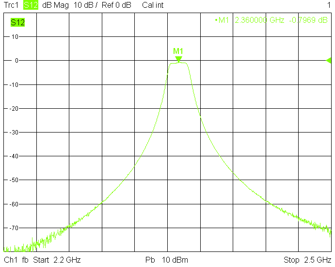
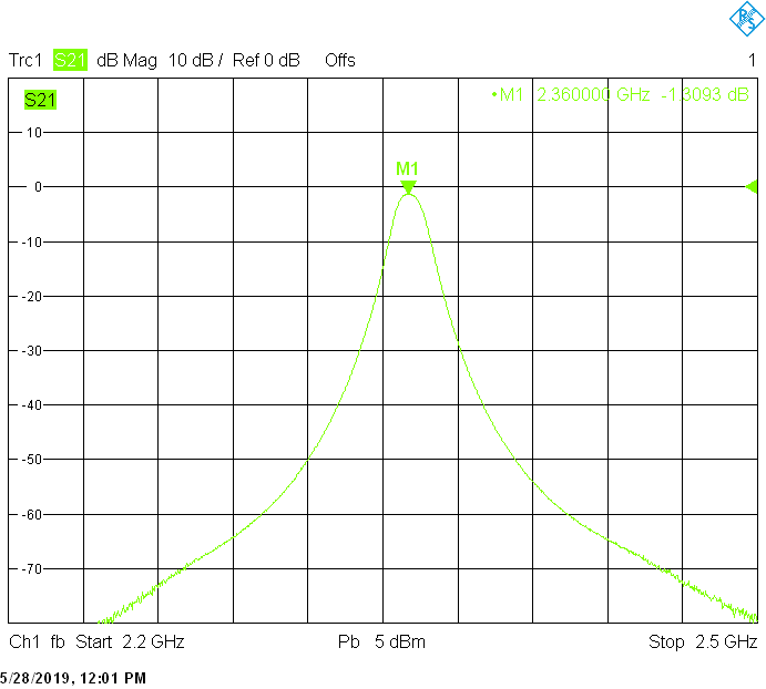
The 140MHz wide version uses 15mm resonator spacing in a rectangular 40mmX20mm tube. Its insertion loss is very low and is mainly due to impedance mismatch:
The 50MHz wide version uses 20mm resonator spacing in a rectangular 40mmX20mm tube. The finite resonator Q already introduces a small insertion loss:
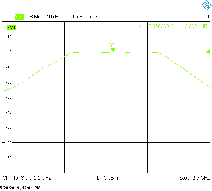
The 30MHz wide version uses 40mm resonator spacing in a rectangular 40mmX30mm tube. The finite resonator Q already introduces a small insertion loss:
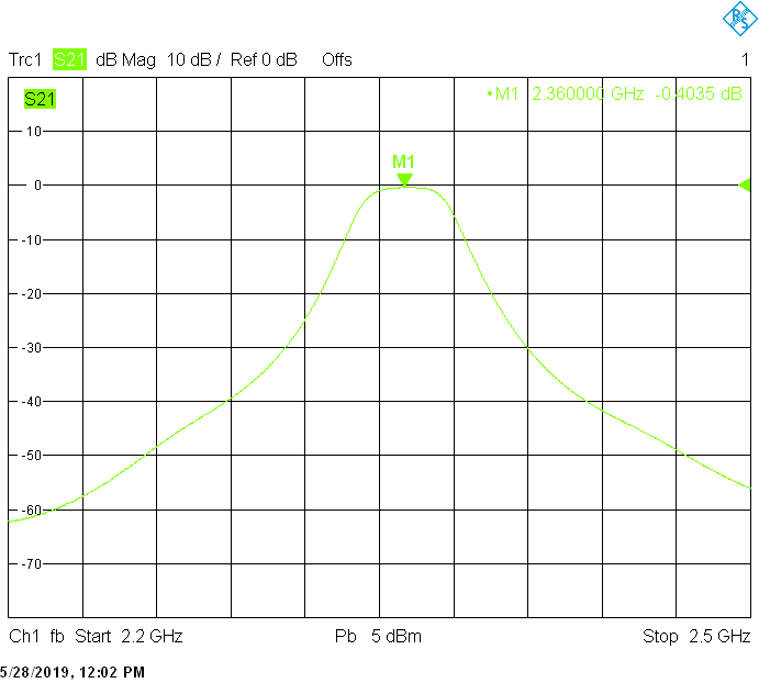
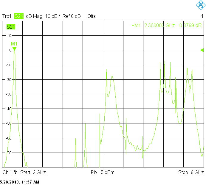
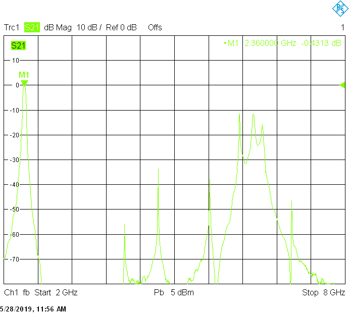
The 20MHz wide version uses 70mm resonator spacing in a square 40mmX40mm tube. Due to the shorter and thicker fingers, longer M3X20 screws may be required for tuning. The finite resonator Q already introduces a small insertion loss:
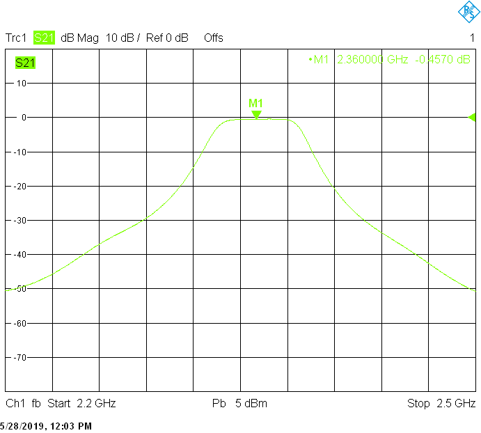
The 10MHz wide version uses 50mm resonator spacing in a rectangular 40mmX30mm tube. The finite resonator Q already introduces a significant insertion loss:
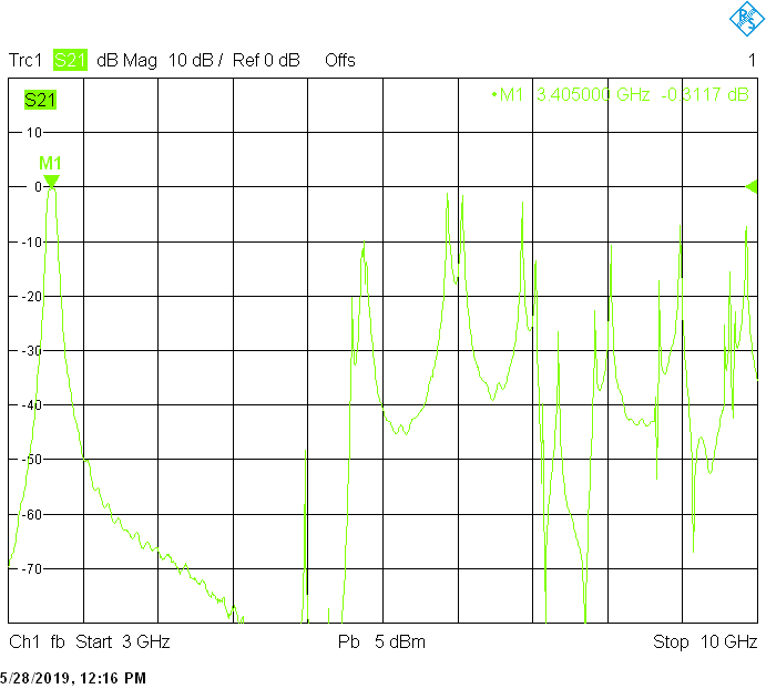
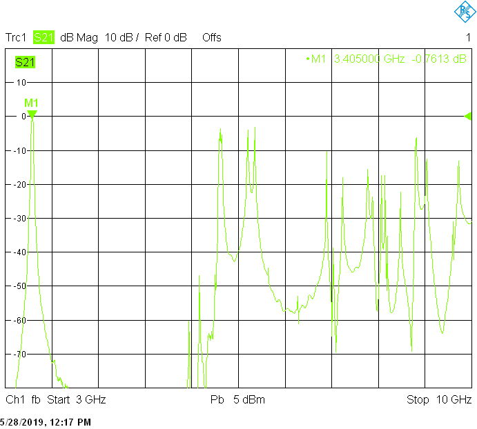
Filters for the 3.4GHz frequency band are built in rectangular aluminum tubes with outside dimensions 30mmX20mm and 30mmX30mm both with 2mm wall thickness:
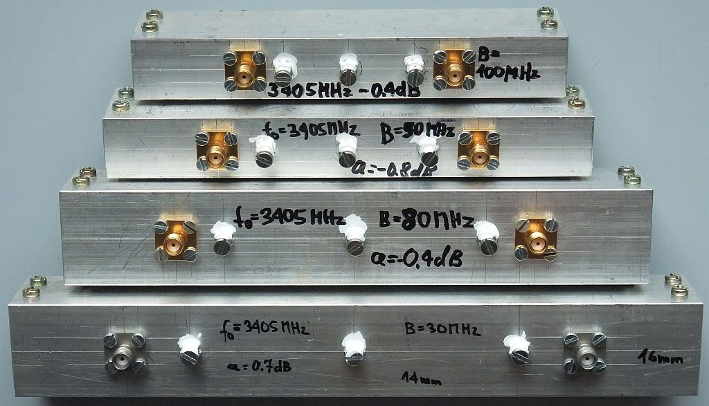
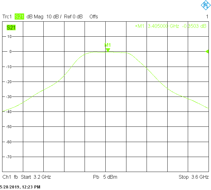
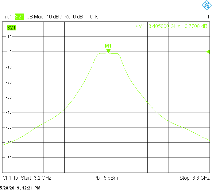
The 100MHz wide version uses 20mm resonator spacing in a rectangular 30mmX20mm tube. The finite resonator Q already introduces a small insertion loss:
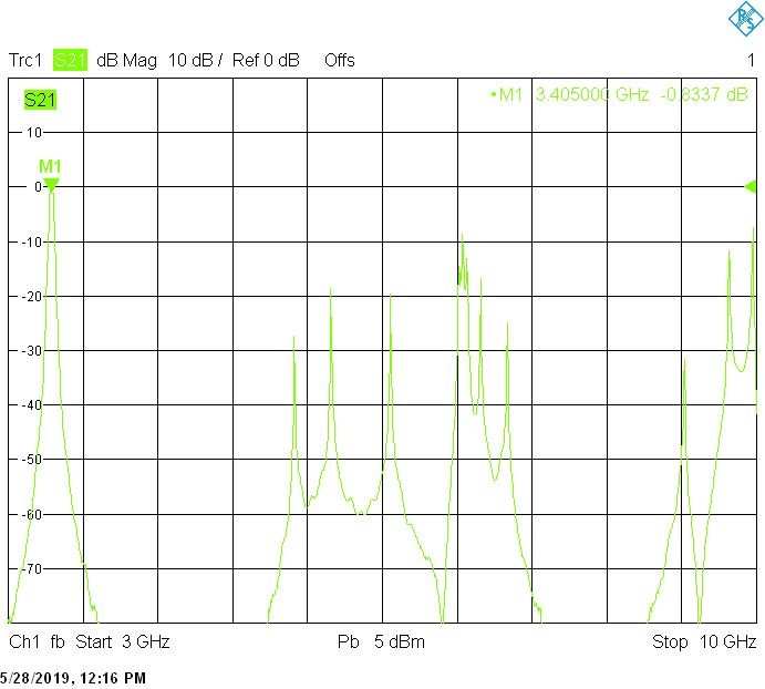
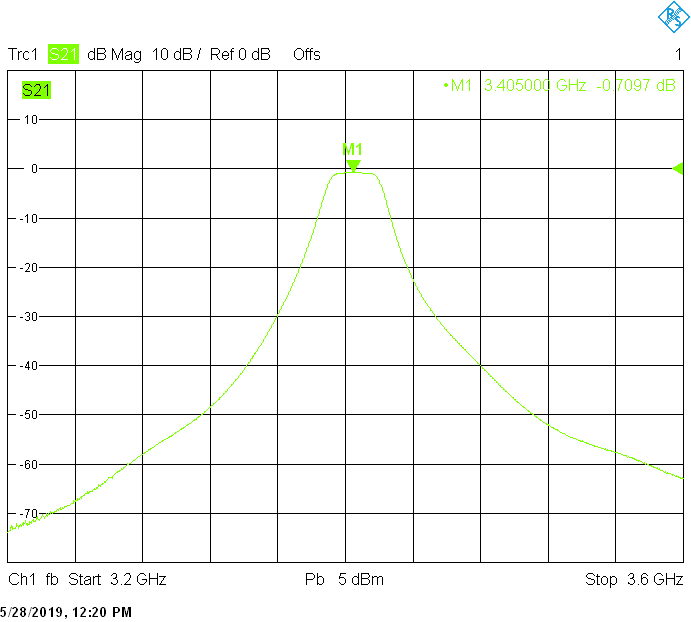
The 80MHz wide version uses 40mm resonator spacing in a square 30mmX30mm tube. The finite resonator Q already introduces a small insertion loss:
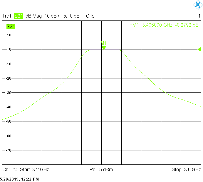
The 50MHz wide version uses 25mm resonator spacing in a rectangular 30mmX20mm tube The finite resonator Q already introduces a considerable insertion loss:
The 30MHz wide version uses 50mm resonator spacing in a square 30mmX30mm tube. The finite resonator Q already introduces a significant insertion loss:
* * * * *